PeakLab v1 Documentation Contents AIST Software Home AIST Software Support
Chromatography Peak Modeling (Tutorial)
For this basic tutorial, we will process and fit four data sets consisting of six cation standards. Three will be processed on a modern instrument, but at various times where a different state of column health might be present, and another where this same standard set was analyzed in 1995. We can then study differences, and also as a matter of interest see how the science of ion chromatography and chromatographic modeling has changed from a quarter century earlier.
Specifically, we want to see how the key a0-a3 chromatographic parameters change across the six peaks in the standard, but also how they change across not only different runs many months apart in time, but across different instruments and decades of time.
Questions
Since one models chromatographic peaks to answer specific questions, let's pose a set of questions before we begin:
(1) What does the S/N look like across the different samples?
(2) How do the actual retention times and estimated plate counts differ across the six peaks, across
the various runs, and across the different eras?
(3) How do the peak widths vary across elution time for the six peaks, and across the various runs
and eras?
(4) How do the intrinsic chromatographic distortions, the fronting and tailing, differ across the
peaks, runs, and eras?
(5) If we can fit a common IRF to all samples, how do the fast system-dependent and slow instrumental
components vary across the four samples?
(6) If we can fit a common generalized model to all samples, what does the non-ideality from the HVL
diffusion theory and NLC kinetic theory look like across the samples and eras?
We will answer all of these questions.
Importing the Data
![]() Click the Open button, the first button in the program's main toolbar. Select the file CationTutorial1.pfd
from the program's installed default data directory (\PeakLab\Data).
Click the Open button, the first button in the program's main toolbar. Select the file CationTutorial1.pfd
from the program's installed default data directory (\PeakLab\Data).
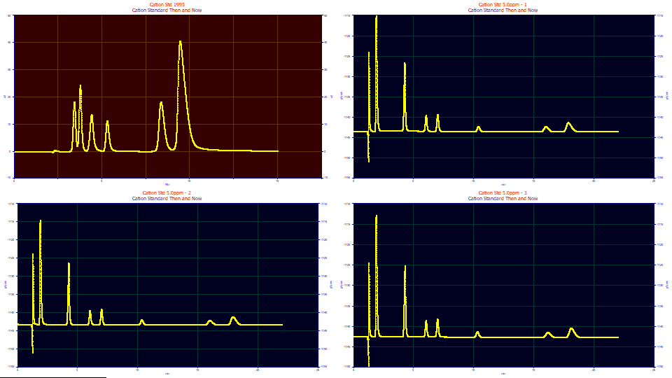
The four data sets are contained in a single PeakLab PFD data file. Each is the raw data from the instrument. The first graph with the red background is the 'principal' data set. Certain functions in the program will apply specifically to this data set. The three graphs with the blue background are 'selected', meaning they will be passed to the visualize and fitting procedures.
Click the second graph using the mouse. It will turn gray, rendering it inaccessible to the visualization and fitting procedures in the program. Click it once again to reselect it so that background is once more blue.
The first step we will take is to put all four graphs on a common retention scale, adjusting for dead-time.
Retention Scale and Dead Time Transforms
![]() The Zoom-in Applies to All Graphs will be on by default. Click this button in the graph's
toolbar to turn this option off. One quick look reveals the dead time in the 1995 data to be just under
2.5 min, where it is about half this value on the three modern samples. We will want to zoom-in the graphs
to see the dead time.
The Zoom-in Applies to All Graphs will be on by default. Click this button in the graph's
toolbar to turn this option off. One quick look reveals the dead time in the 1995 data to be just under
2.5 min, where it is about half this value on the three modern samples. We will want to zoom-in the graphs
to see the dead time.
Using the mouse, zoom-in the dead-time oscillation in each of the four graphs.
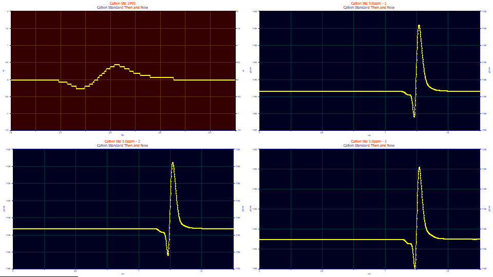
The digitization on the 1995 instrument data is rather apparent.
![]() The Show Graph Hints option will be selected by default. If you move the mouse in the four graphs,
you will see an XY readout of the position of the mouse. Click the Show Graph Hints button. This
is a second level of selection where the hints are synched across the four graphs. We simply want to see
if the three samples from the modern instrument have the same dead time.
The Show Graph Hints option will be selected by default. If you move the mouse in the four graphs,
you will see an XY readout of the position of the mouse. Click the Show Graph Hints button. This
is a second level of selection where the hints are synched across the four graphs. We simply want to see
if the three samples from the modern instrument have the same dead time.
In the second, third, or fourth graph, place the peak at the lowest level of the oscillation which occurs at the dead time. The dead time is identical, 1.23 min for all three peaks. The synch occurs at the x value of the graph you are in with the mouse. We will use this 1.23 min value for the dead time of the three samples. Place the mouse at the similar zone in the first data set. You will see a dead time of 2.18 min.
Normally, we would implement a single transform and do all four data sets at the same time. Here, because of the different values, we must do these adjustments separately.
Right click the first graph and select Apply Transform to this Data Set... from the popup menu. Select the Dead-Time Adjustment for Thermodynamic Capacity Factor from the Common X Transforms dropdown and enter the 2.18 value in the Column Dead Time field. Click OK, Click Accept when the result of the transform is shown in the graph, Yes to accept the local adjustment (there will not be a new transformed data level created in the file, the original data for only this data set will be transformed), and OK to accept the new titles.
Right click the second graph and repeat the procedure above, except use 1.23 for the dead time. Repeat this process for sets three and four using this same 1.23 value.
![]() Click the Titles button in the main toolbar. With Modify Common Elements to All Titles selected,
click All X and enter Retention k', click Apply, and then click OK.
Click the Titles button in the main toolbar. With Modify Common Elements to All Titles selected,
click All X and enter Retention k', click Apply, and then click OK.
Sectioning the Zones of Peaks
Click the Section Data button in the main window. Using the mouse in second graph, box the six peaks to the right. Click Apply in the dialog. The three modern data sets look fine, but we will need to manually section the first data set.
Right click the first graph and select Reset this Data Set - Clear Sectioning. Box the six peaks in this first data set. Click OK, then OK to acknowledge the locally sectioned data set, and OK to acknowledge that this sectioning has been incorporated in this first data level of the file.
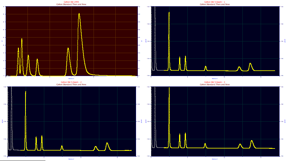
Clearly there are immense differences between the first data set and the other three.
Baseline Correction
Click the Subtract Baseline button in the main window in order to process the baseline in the data sets.
Be sure the following are selected:
Algorithm: 2nd Derivative Zero
Parameters: Sm n 50, Adjust Baseline %, 40
Model: Non-Parm Linear, NP n = 10, Consec = 10
Post Processing: Zero Baseline Points, Zero Negative Points - both unchecked
Graph - Scale Y: Baseline Points
Graph Additional Y - Add D2 to Graphs - unchecked
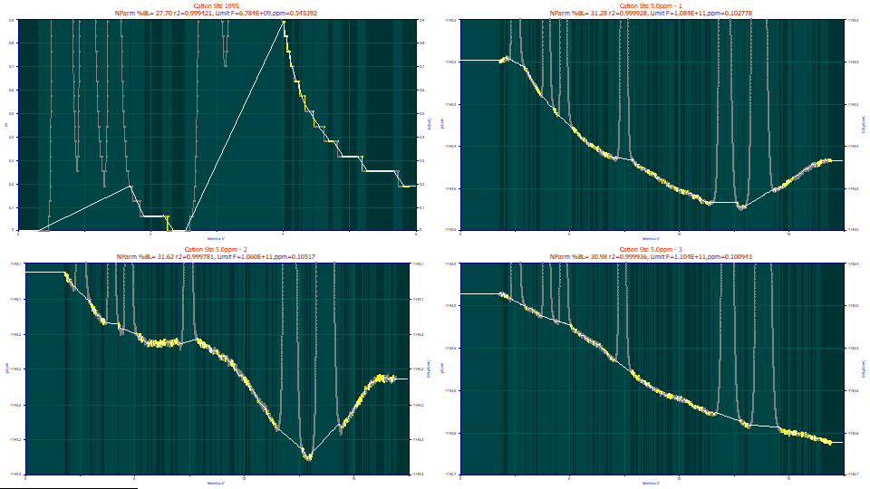
The original scaling will use only the points identified as baseline, allowing a great deal of detail. When fitting peaks to just a few ppm unaccounted variance, the quality of the baseline subtraction is important. It is why this procedure is so extensive, offering multiple methods, models, and adjustments. It takes very little experience to visually know one has a good baseline. We could make some small improvements by manually adjusting the baseline, but this automated procedure should be sufficient for the purposes of this tutorial.
Click on the All Points option. The graphs are now scaled for all of the points.
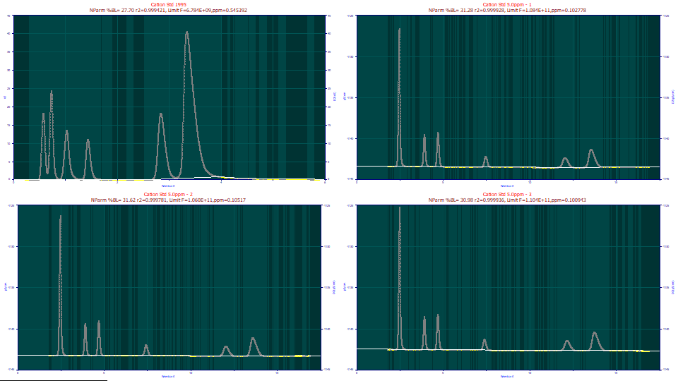
There is information in the title pertaining to the non-parametric modeling and the expected fit statistics if the data assigned to peaks were to exhibit zero error in the fitting, and the only error lay in the baseline variability. You will note that exceptionally good fits are potentially possible even with the 1995 data, or at least the state of the baseline is not disqualifying.
Click OK. Click OK to acknowledge the automatic titles for the new data level. There are now two data levels in the file, the original data with the dead time transforms applied, and the baseline corrected data. The sectioning of the six peaks is inherited and common to both levels.
Visualization
We now have prepared data we can fit, but before we do so, we will use the program's visualization procedure for discrete data.
Click the View and Compare Data button in the main window.
Select Contour if it is not selected.
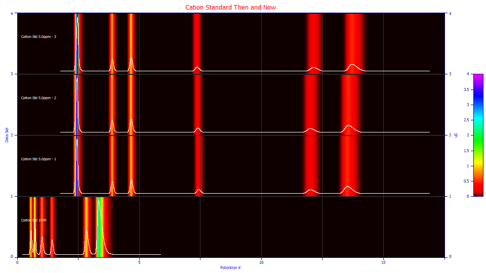
Despite the massive difference in retention values, the widths of the six peaks, on the k' scale, look surprisingly similar. There are subtle differences evident in the three modern sets, mostly positional. You can look at the data with no normalization, or normalized to unit area, or to unit maximum amplitude. Various 3D plots are also available. Feel free to explore the various visualizations. Click OK when you are finished to return to the main window.
Estimating the S/N of the Different Samples
From the main Data menu, select the Fourier Denoising option.
![]() Click the Hide Y2 plot in the graph's toolbar. We will not be filtering the data. We merely wish
to inspect the Fourier spectra of the four different data sets to quantify differences in S/N.
Click the Hide Y2 plot in the graph's toolbar. We will not be filtering the data. We merely wish
to inspect the Fourier spectra of the four different data sets to quantify differences in S/N.
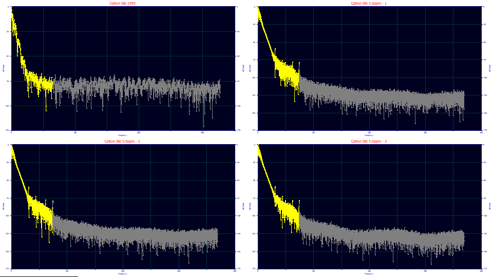
(1) What does the S/N look like across the different samples?
A noise floor is that dB threshold, at higher frequencies, where pure noise, zero signal exists. In the Data Set dropdown, successively select the 4 data sets. The first data set should have a dB threshold noise floor near -83 dB (4.2 digits), the second -128 dB (6.4 digits), the third -127 dB (6.4 digits), and the fourth -129 dB (6.5 digits). In a Fourier decibel plot, 20 dB corresponds to one order of magnitude. Clearly the earlier data has a significantly higher noise. Although the estimate of the noise floor is close to constant across the three modern samples, there are subtle qualitative differences.
This kind of Fourier plot is typical of peak data. Note that the 6.4 digits is the point where all signal is lost. If you look at the frequency where a smooth linear decay begins to become noisy, you can find the other side of the noise estimate, where all is signal and there is no discernible noise. For the first sample, there is noise from the first frequencies, possibly from the digitization of that era. If we look at the second through fourth samples, there is a clean noise-free signal to about -65 dB. This implies the first 3+ digits in the data should be accurate signal, and little impacted by noise.
Click Cancel to exit the Fourier procedure. We do not want to create a new Fourier denoised data level. The fitting process manages the noise in the data.
Fitting the GenNLC<e2> Model
Click the Local Maxima Peaks button. You will use the other two options only if you need help in locating hidden peaks. In these data sets, the peaks are clearly defined by local maxima, each with a distinct apex, and are readily identified and fitted.
You will see the peak placement screen. Ensure the following settings are selected:
Peak Detection
Set Sm
n(1) to 25
Peak Type
Select Chromatography
in the first dropdown
Select GenNLC<e2> as the model in the
second dropdown
Scan
Set the Amp %
threshold to 1.5 %
Leave Use Baseline Segments unchecked
Be sure Use IRF,ZDD is checked
Vary
Leave width a2
and shape a3 checked, all other unchecked
You will note that each of the data sets has an automatic placement of this model with 6 peaks.
Click the IRF button. If you made modifications to the IRF defaults prior to this tutorial for your own fitting, please use the Save button to save your IRF values before resetting the defaults. Click the Defaults button. These are based on retention scale averages of modern IC data for each of the IRFs built into the program.
In a nod to the long sweeping tails of the 1995 data we will fit the IRF that consists of an adjustable area fraction of a fast and slow exponential component, the <e2> IRF.
For modern chromatographic data you will likely find that the half-Gaussian summed with a slow exponential <ge> to be equivalent, and we prefer such since the <ge> may be the better IRF to account the axial dispersion.
There are multiple sources of non-idealities addressed in a system/instrumental IRF, and the fast (narrow width) components can often be adequately fitted with a first order kinetic decay. In fact, the ease at which a two component exponential IRF can be fitted to significance is strongly suggestive that it may actually be the more appropriate IRF. Here will simply note that you will probably find it difficult to distinguish between the <ge> and <e2> IRFs with respect to efficacy. That doesn't mean you can fit a single component exponential IRF successfully. A fast component is necessary.
We will fit the GenNLC<e2> model, a generalized NLC which fits first order adsorption-desorption kinetics, a model very appropriate to IC. You should use a GenNLC model if you wish to fit the kinetics, and a GenHVL model if you want to fit a deconvolved Gaussian SD for the width.
Click the Peak Fit button in the lower left of the dialog to open the fit strategy dialog. Select the Fit with Reduced Data Prefit, Cycle Peaks, 2 Pass, Lock Shared Parameters on Pass 1. Be sure the Fit using Sequential Constraints box checked. Click OK. If you are fitting any peak model bearing an IRF or ZDD parameter(s), you will almost always wish to use a 2-Pass option where the main peak parameters are first estimated while the starting estimates for the IRF and/or ZDD are held constant. If you are fitting multiple peaks, you will almost always wish to use the Cycle Peaks option which performs individual fits of the separate peaks within an overall fit.
Uncheck the Iteration Update button to speed up fitting. This stops the graphical update with each iteration where an improvement in fit occurred.
Because we are fitting an integral (a Fourier convolution) to each peak, and using a complex strategy involving as many as forty distinct fits within an overall fit of data set, and we have four data sets, the fits will require some time, perhaps a minute or so. Click Review Fit when the fitting is finished.
Reviewing the Fit
Your goodness of fit values will be slightly different since we manually sectioned the active points to be fitted using the mouse.
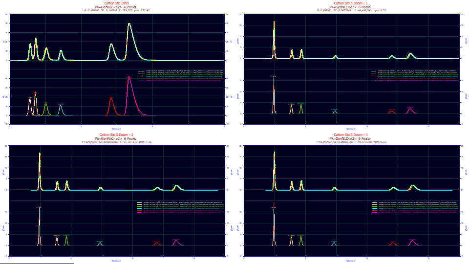
In our case, we have 257 ppm unaccounted variance in the 1995 data. The three modern sets have values ranging from 7.2-8.3 ppm unaccounted variance. A ppm of 8 corresponds with an r2 goodness of fit of 0.999992. The best we achieved with prior versions of the product, where no IRF convolution integral fitting was available, was about 3500 ppm. Such refinements in the accuracy of fitting are important for the higher moment parameters of a model as well as IRF parameters and estimates of deviation from the theoretical expectations of chromatographic shapes.
![]() The Zoom-in Applies to All Graphs will in on by default. Click this button in the graph's
toolbar to turn this option off. We need to zoom the graphs independently to manage the different scales
in the data sets.
The Zoom-in Applies to All Graphs will in on by default. Click this button in the graph's
toolbar to turn this option off. We need to zoom the graphs independently to manage the different scales
in the data sets.
Using the mouse, zoom-in different peaks in the upper graphs. To restore the full scaling, right click a graph and select the Restore Scaling - Undo Zoom option.
![]() You can use the Hide Y plot in the graph's toolbar to see just the upper plot.
You can use the Hide Y plot in the graph's toolbar to see just the upper plot.
To see just a single data set, double click that graph. Double click that graph once more to restore all plots. You can also use the right click popup menu.
(2) How do the actual retention times and estimated plate counts differ across the six peaks, across the various runs, and across the different eras?
Click Numeric. In the Options menu of the Numeric Summary, choose Select Only Fitted Parameters, check the Chromatography Analysis option, and uncheck the Fitted Parameters option:
"Cation Std 1995"
"Pk=GenNLC<e2> 6 Peaks "
"r2=0.999742 SE=0.116808 F=522,879 ppm=257.84"
"Retention k'"
"uS"
Chromatographic Analysis
Peak Type N-moment N-Gauss FW Base Asym10 Resolution Retention
1 GenNLC<e2> 63.4537336 352.213948 0.14571788 1.12590347 0.55482628
2 GenNLC<e2> 103.350443 649.709159 0.13686961 1.05028287 1.10785172 0.71058006
3 GenNLC<e2> 171.482355 583.867681 0.20537058 1.23245872 1.70494303 1.01089070
4 GenNLC<e2> 347.494527 1374.10030 0.19066769 1.52691527 2.06102161 1.44549791
5 GenNLC<e2> 951.521786 2020.31701 0.31437494 1.73910896 5.57022373 2.88825297
6 GenNLC<e2> 823.178563 1435.37971 0.45744003 3.08978259 1.29635447 3.53318782
"Cation Std 5.0ppm - 1"
"Pk=GenNLC<e2> 6 Peaks "
"r2=0.999992 SE=0.00354176 F=50,808,324 ppm=8.28"
"Retention k'"
"ﭖS/cm"
Chromatographic Analysis
Peak Type N-moment N-Gauss FW Base Asym10 Resolution Retention
1 GenNLC<e2> 2266.96002 3819.15923 0.21642302 0.82625246 2.38119505
2 GenNLC<e2> 4633.30798 6069.43562 0.25126407 1.14439293 6.18232075 3.87310422
3 GenNLC<e2> 6033.73771 7540.65439 0.26755270 1.16350757 3.01647361 4.66041706
4 GenNLC<e2> 7930.87337 8509.55310 0.38638754 1.17364614 8.43547062 7.43427195
5 GenNLC<e2> 6706.46590 6852.63710 0.68725901 1.34400767 8.51939084 12.0851582
6 GenNLC<e2> 6525.62344 6877.48526 0.77751117 1.71996531 2.06376415 13.7089331
"Cation Std 5.0ppm - 2"
"Pk=GenNLC<e2> 6 Peaks "
"r2=0.999993 SE=0.00333791 F=58,235,637 ppm=7.23"
"Retention k'"
"ﭖS/cm"
Chromatographic Analysis
Peak Type N-moment N-Gauss FW Base Asym10 Resolution Retention
1 GenNLC<e2> 2309.57851 3829.28167 0.21492596 0.81025435 2.38421480
2 GenNLC<e2> 4675.30993 6069.97603 0.25022167 1.13270477 6.17581374 3.86682770
3 GenNLC<e2> 6076.93803 7539.82101 0.26638780 1.15416843 3.01073402 4.64942543
4 GenNLC<e2> 7882.35894 8435.58574 0.38602116 1.16656388 8.37905374 7.39798358
5 GenNLC<e2> 6705.79603 6858.25445 0.68725595 1.34937204 8.58969234 12.0871593
6 GenNLC<e2> 6561.18466 6928.39093 0.77772476 1.72412332 2.12212609 13.7533018
"Cation Std 5.0ppm - 3"
"Pk=GenNLC<e2> 6 Peaks "
"r2=0.999992 SE=0.00364019 F=50,498,222 ppm=8.33"
"Retention k'"
"ﭖS/cm"
Chromatographic Analysis
Peak Type N-moment N-Gauss FW Base Asym10 Resolution Retention
1 GenNLC<e2> 2332.49616 3990.34736 0.21347864 0.79855784 2.40141373
2 GenNLC<e2> 4691.85133 6198.24799 0.24867989 1.12703222 6.16116733 3.87189625
3 GenNLC<e2> 6052.48793 7595.24705 0.26604866 1.14972258 3.01339525 4.65255014
4 GenNLC<e2> 7804.99899 8386.47799 0.38554224 1.16559613 8.27098165 7.36294375
5 GenNLC<e2> 6802.28734 6947.82469 0.68938270 1.35955873 8.87458900 12.2167423
6 GenNLC<e2> 6606.56475 6957.16242 0.78361340 1.74456006 2.14660938 13.9124937
The retention values are about 4x higher on the modern data. The capacity factors that spanned from .55 to 3.5 in this earlier era now span from 2.4 to 13.8. The theoretical plate count, by method of moments, is vastly improved. The 63-951 plates of the earlier era data range from 2260-7900 in the modern data. The three modern samples of the standard show a remarkable constancy across the better part of a year's time.
In the Options menu of the Numeric Summary, choose Select Only Fitted Parameters:
"Cation Std 1995"
Fitted Parameters
r2 Coef Det DF Adj r2 Fit Std Err F-value ppm uVar
0.99974216 0.99974018 0.11680750 522,879 257.835680
Peak Type a0 a1 a2 a3 a4 a5 a6 a7
1 GenNLC<e2> 1.46897112 0.55482628 0.00067629 -0.0019405 2.42563915 0.00599348 0.15521158 0.89594172
2 GenNLC<e2> 1.80999115 0.71058006 0.00047704 -0.0013915 2.42563915 0.00599348 0.15521158 0.89594172
3 GenNLC<e2> 1.45001342 1.01089070 0.00080430 -0.0008358 2.42563915 0.00599348 0.15521158 0.89594172
4 GenNLC<e2> 1.12264255 1.44549791 0.00051413 0.00140432 2.42563915 0.00599348 0.15521158 0.89594172
5 GenNLC<e2> 2.99811154 2.88825297 0.00069184 0.00323794 2.42563915 0.00599348 0.15521158 0.89594172
6 GenNLC<e2> 9.22053157 3.53318782 0.00108274 0.01516076 2.42563915 0.00599348 0.15521158 0.89594172
"Cation Std 5.0ppm - 1"
Fitted Parameters
r2 Coef Det DF Adj r2 Fit Std Err F-value ppm uVar
0.99999172 0.99999170 0.00354176 50,808,324 8.28233042
Peak Type a0 a1 a2 a3 a4 a5 a6 a7
1 GenNLC<e2> 1.78783058 2.38119505 0.00023937 -0.0023288 1.37441970 0.00641836 0.04439327 0.59945320
2 GenNLC<e2> 0.49931902 3.87310422 0.00027190 -0.0003735 1.37441970 0.00641836 0.04439327 0.59945320
3 GenNLC<e2> 0.57450105 4.66041706 0.00026513 -0.0001887 1.37441970 0.00641836 0.04439327 0.59945320
4 GenNLC<e2> 0.26051189 7.43427195 0.00039251 0.00029174 1.37441970 0.00641836 0.04439327 0.59945320
5 GenNLC<e2> 0.43996937 12.0851582 0.00082895 0.00271512 1.37441970 0.00641836 0.04439327 0.59945320
6 GenNLC<e2> 0.90270041 13.7089331 0.00089076 0.00616536 1.37441970 0.00641836 0.04439327 0.59945320
"Cation Std 5.0ppm - 2"
Fitted Parameters
r2 Coef Det DF Adj r2 Fit Std Err F-value ppm uVar
0.99999277 0.99999276 0.00333791 58,235,637 7.22601811
Peak Type a0 a1 a2 a3 a4 a5 a6 a7
1 GenNLC<e2> 1.79821792 2.38421480 0.00023819 -0.0023401 1.46295365 0.00638164 0.04399482 0.61116432
2 GenNLC<e2> 0.50251890 3.86682770 0.00027285 -0.0003907 1.46295365 0.00638164 0.04399482 0.61116432
3 GenNLC<e2> 0.58257824 4.64942543 0.00026597 -0.0002024 1.46295365 0.00638164 0.04399482 0.61116432
4 GenNLC<e2> 0.26356445 7.39798358 0.00039597 0.00026536 1.46295365 0.00638164 0.04399482 0.61116432
5 GenNLC<e2> 0.44378173 12.0871593 0.00083112 0.00274450 1.46295365 0.00638164 0.04399482 0.61116432
6 GenNLC<e2> 0.90779499 13.7533018 0.00089168 0.00616605 1.46295365 0.00638164 0.04399482 0.61116432
"Cation Std 5.0ppm - 3"
Fitted Parameters
r2 Coef Det DF Adj r2 Fit Std Err F-value ppm uVar
0.99999167 0.99999165 0.00364019 50,498,222 8.33319053
Peak Type a0 a1 a2 a3 a4 a5 a6 a7
1 GenNLC<e2> 1.82083536 2.40141373 0.00023444 -0.0023516 1.15585607 0.00609074 0.04503216 0.62477753
2 GenNLC<e2> 0.50969105 3.87189625 0.00026905 -0.0003941 1.15585607 0.00609074 0.04503216 0.62477753
3 GenNLC<e2> 0.59166151 4.65255014 0.00026525 -0.0002013 1.15585607 0.00609074 0.04503216 0.62477753
4 GenNLC<e2> 0.26712356 7.36294375 0.00039605 0.00028201 1.15585607 0.00609074 0.04503216 0.62477753
5 GenNLC<e2> 0.44992976 12.2167423 0.00082209 0.00288149 1.15585607 0.00609074 0.04503216 0.62477753
6 GenNLC<e2> 0.92357664 13.9124937 0.00088263 0.00636716 1.15585607 0.00609074 0.04503216 0.62477753
(3) How do the kinetic rates and peak widths vary across elution time for the six peaks, and across the various runs and eras?
The a2 in the NLC parameterization is a time constant instead of a rate constant. The kinetics fit to about 3x faster on the modern data for the first three fronted peaks, and are close to the same for the last of the tailed peaks. The a2 parameters appear quite stable across the three modern data sets. The kinetic rates diminish (the a2 time constants increase) with elution time on both the historical and modern data. The increase in a2 across the peaks is actually higher on the modern data with longer elution times.
(4) How do the intrinsic chromatographic distortions, the fronting and tailing, differ across the peaks, runs, and eras?
The fronting and tailing is consistent across the two different eras; the first three peaks fronted (-a3), and the last three peaks tailed (+a3). We have to confess this was probably the most surprising of the results, given the vast differences in a quarter century of instrumentation, columns, and detectors. Even more amazing, if we look at the first and fifth peaks underlined above, we see very close to the same a3 distortions across the different eras. There are certainly differences, but the fronting to tailing is as consistent in the 1990's data as that of present time. The a3 parameters also appear very stable across the three modern data sets.
(5) If we can fit a common IRF to all samples, how do the fast system-dependent and slow instrumental components vary across the four samples?
With respect to the instrumental/system IRF, here fitted as a fast and slow exponential, there is one overriding observation. The a6 slow exponential, the component responsible for most of the visual tailing, probably detector related since it fits largely independent of system variables, is 4x higher in the earlier era. The a5 fits to statistical significance (although only weakly so), and the fits suggest a greater proportion of this fast component, 90% vs. 60%, in the earlier data. There is, however, no difference in the actual value of the narrow width. There are modest differences in the IRF parameters in the three modern data fits, possibly related to column health. We have some evidence that diminished column health is reflected mostly in the IRF (the additional tailing that adds upon the intrinsic peak shape) and in the ZDD zero-distortion density's higher moment adjustments.
(6) If we can fit a common generalized model to all samples, what does the non-ideality from the HVL diffusion theory and NLC kinetic theory look like across the samples and eras?
The most telling difference is with a4, the third moment or skewness adjustment, in its deviation from theoretical shape. A pure HVL peak has a Gaussian zero-distortion (infinite dilution) density, or ZDD, with an a4=0, zero asymmetry. A pure NLC shape has a Giddings ZDD with an a4=0.5, a slight right-skewed asymmetry. Here we do see a good a4 significance in the fits, and there are appreciable differences between the three states of the column in the modern instrument. The third of the three modern sets fits closer to this 0.5 ideality of shape, 1.15 as contrasted with the 1.38 and 1.46 of the first two sets. In all cases, we have a greater infinite dilution asymmetry than the pure theoretical kinetics of the NLC would predict. For the earlier era instrument and column, we have an a4 of 2.42, a much greater deviation from theoretical ideality. This is a trend we've observed in many data sets. As technologies improve, the deviations from this a4 ideal expectation have become smaller.
In the Options menu of the Numeric Summary, check the Measured Values, Equivalent Parameters, and Average Multiple Fits:
Only identical fits (those which use the same model, have same count of peaks, and are fitted identically) are available for averaging. We will first take note of the older era fit:
"Cation Std 1995"
Fitted Parameters
r2 Coef Det DF Adj r2 Fit Std Err F-value ppm uVar
0.99974216 0.99974018 0.11680750 522,879 257.835680
Peak Type a0 a1 a2 a3 a4 a5 a6 a7
1 GenNLC<e2> 1.46897112 0.55482628 0.00067629 -0.0019405 2.42563915 0.00599348 0.15521158 0.89594172
2 GenNLC<e2> 1.80999115 0.71058006 0.00047704 -0.0013915 2.42563915 0.00599348 0.15521158 0.89594172
3 GenNLC<e2> 1.45001342 1.01089070 0.00080430 -0.0008358 2.42563915 0.00599348 0.15521158 0.89594172
4 GenNLC<e2> 1.12264255 1.44549791 0.00051413 0.00140432 2.42563915 0.00599348 0.15521158 0.89594172
5 GenNLC<e2> 2.99811154 2.88825297 0.00069184 0.00323794 2.42563915 0.00599348 0.15521158 0.89594172
6 GenNLC<e2> 9.22053157 3.53318782 0.00108274 0.01516076 2.42563915 0.00599348 0.15521158 0.89594172
Equivalent Parameters
Peak Type a0 a1 a2 a3 a4 a5 a6 a7
1 GenHVL<e2> 1.46897112 0.55482628 0.02739429 -0.0019405 0.11976480 0.00599348 0.15521158 0.89594172
2 GenHVL<e2> 1.80999115 0.71058006 0.02603759 -0.0013915 0.08888201 0.00599348 0.15521158 0.89594172
3 GenHVL<e2> 1.45001342 1.01089070 0.04032520 -0.0008358 0.09676058 0.00599348 0.15521158 0.89594172
4 GenHVL<e2> 1.12264255 1.44549791 0.03855333 0.00140432 0.06469498 0.00599348 0.15521158 0.89594172
5 GenHVL<e2> 2.99811154 2.88825297 0.06321731 0.00323794 0.05309174 0.00599348 0.15521158 0.89594172
6 GenHVL<e2> 9.22053157 3.53318782 0.08747036 0.01516076 0.06005102 0.00599348 0.15521158 0.89594172
Measured Values
Peak Type Amplitude Center FWHM Asym50 FW Base Asym10
1 GenNLC<e2> 18.0664641 0.57183758 0.07175087 0.99016625 0.14571788 1.12590347
2 GenNLC<e2> 23.6579938 0.72837010 0.06728997 0.95283961 0.13686961 1.05028287
3 GenNLC<e2> 12.9473148 1.02012012 0.09941498 1.07241034 0.20537058 1.23245872
4 GenNLC<e2> 10.9001746 1.42824184 0.09072987 1.29582020 0.19066769 1.52691527
5 GenNLC<e2> 18.0913150 2.83484206 0.14851723 1.45126162 0.31437494 1.73910896
6 GenNLC<e2> 40.0110540 3.33511495 0.20729325 2.35041641 0.45744003 3.08978259
Peak Type Area % Area Mean StdDev Skewness Kurtosis
1 GenNLC<e2> 1.46897113 8.12921899 0.58758163 0.07376318 5.04216941 43.3129083
2 GenNLC<e2> 1.80999116 10.0164082 0.74284426 0.07307042 5.18024623 44.8624600
3 GenNLC<e2> 1.45001345 8.02430803 1.03825405 0.07928553 4.08270720 33.2072957
4 GenNLC<e2> 1.12264258 6.21265262 1.45233454 0.07790991 4.31670545 35.4021723
5 GenNLC<e2> 2.99811156 16.5914121 2.86959442 0.09302746 2.65852328 18.9826398
6 GenNLC<e2> 9.22053165 51.0260000 3.41325252 0.11896560 1.64437704 9.16174028
All Total 18.0702615 100.000000
The averages will initially include all four of the fits. Highlight fit 2, 3, and 4 by left clicking the second through fourth graphs. Each graph will now have a gray outline. Right click any graph and select Plot | Only Selected Fits. Only three fits are now graphed and the averages in the Numeric Summary reflect only the three modern data sets. Scroll to the bottom of the summary to view the Average and CV% sections:
Average for 3 Fits
Fitted Parameters
r2 Coef Det DF Adj r2 Fit Std Err F-value ppm uVar
0.99999205 0.99999203 0.00350662 53,180,728 7.94717969
Peak Type a0 a1 a2 a3 a4 a5 a6 a7
1 GenNLC<e2> 1.80229462 2.38894119 0.00023733 -0.0023401 1.33107647 0.00629691 0.04447341 0.61179835
2 GenNLC<e2> 0.50384299 3.87060939 0.00027127 -0.0003861 1.33107647 0.00629691 0.04447341 0.61179835
3 GenNLC<e2> 0.58291360 4.65413087 0.00026545 -0.0001975 1.33107647 0.00629691 0.04447341 0.61179835
4 GenNLC<e2> 0.26373330 7.39839976 0.00039485 0.00027970 1.33107647 0.00629691 0.04447341 0.61179835
5 GenNLC<e2> 0.44456029 12.1296866 0.00082739 0.00278037 1.33107647 0.00629691 0.04447341 0.61179835
6 GenNLC<e2> 0.91135735 13.7915762 0.00088836 0.00623286 1.33107647 0.00629691 0.04447341 0.61179835
Equivalent Parameters
Peak Type a0 a1 a2 a3 a4 a5 a6 a7
1 GenHVL<e2> 1.80229462 2.38894119 0.03367361 -0.0023401 0.01877289 0.00629691 0.04447341 0.61179835
2 GenHVL<e2> 0.50384299 3.87060939 0.04582480 -0.0003861 0.01576372 0.00629691 0.04447341 0.61179835
3 GenHVL<e2> 0.58291360 4.65413087 0.04970785 -0.0001975 0.01421704 0.00629691 0.04447341 0.61179835
4 GenHVL<e2> 0.26373330 7.39839976 0.07643528 0.00027970 0.01374948 0.00629691 0.04447341 0.61179835
5 GenHVL<e2> 0.44456029 12.1296866 0.14167373 0.00278037 0.01555439 0.00629691 0.04447341 0.61179835
6 GenHVL<e2> 0.91135735 13.7915762 0.15653420 0.00623286 0.01511557 0.00629691 0.04447341 0.61179835
Measured Values
Peak Type Amplitude Center FWHM Asym50 FW Base Asym10
1 GenNLC<e2> 16.9478203 2.45981898 0.09300735 0.65948892 0.21494254 0.81168822
2 GenNLC<e2> 3.89282253 3.89506777 0.11732129 1.00308265 0.25005521 1.13470997
3 GenNLC<e2> 4.20062927 4.67364300 0.12658885 1.03514076 0.26666305 1.15579953
4 GenNLC<e2> 1.29371808 7.40233629 0.18969526 1.09392267 0.38598365 1.16860205
5 GenNLC<e2> 1.21891571 12.0532449 0.34203498 1.25219719 0.68796589 1.35097948
6 GenNLC<e2> 2.21858949 13.6022051 0.38501734 1.52581564 0.77961644 1.72954957
Peak Type Area % Area Mean StdDev Skewness Kurtosis
1 GenNLC<e2> 1.80229035 39.9741326 2.45363321 0.05113008 0.72947750 5.74522024
2 GenNLC<e2> 0.50384312 11.1749581 3.90085629 0.05710238 0.63917239 4.76812846
3 GenNLC<e2> 0.58291316 12.9283025 4.68039789 0.06015194 0.56479292 4.43688655
4 GenNLC<e2> 0.26373343 5.84937743 7.41182181 0.08353402 0.28276020 3.39370049
5 GenNLC<e2> 0.44456043 9.86004544 12.0846536 0.14721871 0.29184352 3.08551079
6 GenNLC<e2> 0.91135678 20.2131838 13.6661001 0.16867191 0.46519817 3.11927690
All Total 4.50869729 100.000000
We will first note that the FWHM, full width at half maximum values are actually higher for the modern data, this for each of the six peaks. The kinetic rates are higher for the modern instrument and column, but the longer elutions result in higher peak widths.
Note the exceptionally high skewness and kurtosis (fat tails) in the old era data.
For this first tutorial, we will only make note of the <e2> parameter values of [0.006304, .04447, .6117]. Although there were only three samples averaged, coefficient variation % (CV%) were 3.41, 1.81, and 2.12% for the three parameters. The IRF values were reasonably close across the three fits.
Click OK. All plots, the four fit graphs, are restored. Click OK to close the Review. Check Save updated information to the current data file when adding fits and click OK, accepting the default name for the fit. Click OK to confirm and click OK one last time to leave the placement screen and return to main screen.
Deconvolving the IRF and Fitting a Closed Form Model
When the instrument/system IRF has been accurately determined, you will probably wish to deconvolve the IRF prior to fitting. This allows the fitting of a closed form model which will be exceptionally fast, and there will be no complications associated with fitting the IRF in more complex or messy data.
Click on the IRF Deconvolution button. Ensure the following settings are selected:
Response Fn
<e2> Exponential
Deconvolve Right
Genetic Alg Optimization
These will not be used
Fourier Filter
D2 Automatic (the FFT threshold will be determined
using a smoothed 2nd derivative)
8 (8% smoothing for the D2 algorithm)
Post-Processing
Zero Baseline Points - unchecked (baseline will be
actual subtracted values)
Zero Negative Points - unchecked (negative
baseline points are permitted)
Click the Import from Fit button. Click the Custom Average in the Import IRF Model and Parameters from Fit section. Click the last three <e2> fits. Click OK to accept the selections. Click OK to close the dialog. This will average the values from the three modern data sets updating the IRF model and parameter values in the dialog. You should see the <e2> IRF and values similar to 0.0063, 0.04447, and 0.6118 in the three fields, matching the values from the averages above.
The first data set clearly cannot use this modern-era IRF. Double click the first graph. Enter .005993, .1552, and .8959 from the fit for the three <e2> IRF values. Click OK. The blue background on the graph indicates a custom (local) deconvolution.
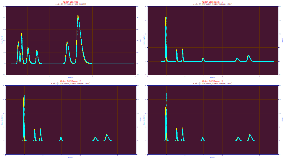
Click OK. Click OK to confirm to acknowledge the local convolution warning. Click OK to accept the default names for the data level and its graph titles.
Fitting the Closed Form GenNLC Model
Click the Local Maxima Peaks button. You will use the other two options only if you need help in locating hidden peaks. In these data sets, the peaks are clearly defined by local maxima, each with a distinct apex, and are readily identified and fitted.
You will see the peak placement screen. Ensure the following settings are selected:
Peak Detection
Set Sm
n(1) to 25
Peak Type
Select Chromatography
in the first dropdown
Select GenNLC as the model in the second dropdown
Scan
Set the Amp %
threshold to 1.5 %
Leave Use Baseline Segments unchecked
Be sure Use IRF,ZDD is checked
Vary
Leave width a2
and shape a3 checked, all other unchecked
Click the Peak Fit button in the lower left of the dialog to open the fit strategy dialog. Select the Fit with Reduced Data Prefit, Cycle Peaks, 2 Pass, Lock Shared Parameters on Pass 1. Be sure the Fit using Sequential Constraints box checked. Click OK. The fits should require only a second or two.
Click Review Fit.
The goodness of fit will be somewhat weaker since the IRF is no longer exactly modeled in any of the fits. The old era data fits to about 301 ppm, the three modern data sets fit to about 47.8, 20.6, and 21.0 ppm.
Click Numeric. In the Options menu of the Numeric Summary, choose Select Only Fitted Parameters:
Fitting an IRF Convolution Model vs. Subtracting an IRF Prior to Fitting a Closed Form Model
We'll compare the fits of of the pre-deconvolved data with the direct IRF fits:
"Cation Std 1995"
Fitted Parameters
r2 Coef Det DF Adj r2 Fit Std Err F-value ppm uVar
0.99969821 0.99969614 0.13284404 502,965 301.785221
Peak Type a0 a1 a2 a3 a4
1 GenNLC 1.45866820 0.55598378 0.00067979 -0.0018889 2.42307652
2 GenNLC 1.80271255 0.71182392 0.00048155 -0.0013431 2.42307652
3 GenNLC 1.44770735 1.01139865 0.00081095 -0.0008738 2.42307652
4 GenNLC 1.11940089 1.44672894 0.00051943 0.00144234 2.42307652
5 GenNLC 2.98838529 2.89062705 0.00069736 0.00334746 2.42307652
6 GenNLC 9.20949876 3.53632684 0.00109387 0.01542843 2.42307652
Fitted Parameters
r2 Coef Det DF Adj r2 Fit Std Err F-value ppm uVar
0.99974216 0.99974018 0.11680750 522,879 257.835680
Peak Type a0 a1 a2 a3 a4 a5 a6 a7
1 GenNLC<e2> 1.46897112 0.55482628 0.00067629 -0.0019405 2.42563915 0.00599348 0.15521158 0.89594172
2 GenNLC<e2> 1.80999115 0.71058006 0.00047704 -0.0013915 2.42563915 0.00599348 0.15521158 0.89594172
3 GenNLC<e2> 1.45001342 1.01089070 0.00080430 -0.0008358 2.42563915 0.00599348 0.15521158 0.89594172
4 GenNLC<e2> 1.12264255 1.44549791 0.00051413 0.00140432 2.42563915 0.00599348 0.15521158 0.89594172
5 GenNLC<e2> 2.99811154 2.88825297 0.00069184 0.00323794 2.42563915 0.00599348 0.15521158 0.89594172
6 GenNLC<e2> 9.22053157 3.53318782 0.00108274 0.01516076 2.42563915 0.00599348 0.15521158 0.89594172
"Cation Std 5.0ppm - 1"
Fitted Parameters
r2 Coef Det DF Adj r2 Fit Std Err F-value ppm uVar
0.99995221 0.99995210 0.00926065 9,907,447 47.7942514
Peak Type a0 a1 a2 a3 a4
1 GenNLC 1.78064961 2.38426937 0.00024969 -0.0022751 1.13650007
2 GenNLC 0.49815122 3.87657816 0.00027659 -0.0003019 1.13650007
3 GenNLC 0.57358971 4.66398511 0.00026933 -0.0001218 1.13650007
4 GenNLC 0.26025242 7.43762202 0.00039500 0.00034717 1.13650007
5 GenNLC 0.43984421 12.0888348 0.00082739 0.00278695 1.13650007
6 GenNLC 0.90236656 13.7120585 0.00088509 0.00619670 1.13650007
Fitted Parameters
r2 Coef Det DF Adj r2 Fit Std Err F-value ppm uVar
0.99999172 0.99999170 0.00354176 50,808,324 8.28233042
Peak Type a0 a1 a2 a3 a4 a5 a6 a7
1 GenNLC<e2> 1.78783058 2.38119505 0.00023937 -0.0023288 1.37441970 0.00641836 0.04439327 0.59945320
2 GenNLC<e2> 0.49931902 3.87310422 0.00027190 -0.0003735 1.37441970 0.00641836 0.04439327 0.59945320
3 GenNLC<e2> 0.57450105 4.66041706 0.00026513 -0.0001887 1.37441970 0.00641836 0.04439327 0.59945320
4 GenNLC<e2> 0.26051189 7.43427195 0.00039251 0.00029174 1.37441970 0.00641836 0.04439327 0.59945320
5 GenNLC<e2> 0.43996937 12.0851582 0.00082895 0.00271512 1.37441970 0.00641836 0.04439327 0.59945320
6 GenNLC<e2> 0.90270041 13.7089331 0.00089076 0.00616536 1.37441970 0.00641836 0.04439327 0.59945320
"Cation Std 5.0ppm - 2"
Fitted Parameters
r2 Coef Det DF Adj r2 Fit Std Err F-value ppm uVar
0.99997935 0.99997930 0.00614471 22,928,122 20.6528851
Peak Type a0 a1 a2 a3 a4
1 GenNLC 1.79507988 2.38626356 0.00024399 -0.0023097 1.33884257
2 GenNLC 0.50194619 3.86910957 0.00027522 -0.0003498 1.33884257
3 GenNLC 0.58225926 4.65174577 0.00026822 -0.0001648 1.33884257
4 GenNLC 0.26342823 7.40007002 0.00039680 0.00029367 1.33884257
5 GenNLC 0.44366527 12.0894765 0.00082948 0.00278330 1.33884257
6 GenNLC 0.90756654 13.7553597 0.00088798 0.00618437 1.33884257
Fitted Parameters
r2 Coef Det DF Adj r2 Fit Std Err F-value ppm uVar
0.99999277 0.99999276 0.00333791 58,235,637 7.22601811
Peak Type a0 a1 a2 a3 a4 a5 a6 a7
1 GenNLC<e2> 1.79821792 2.38421480 0.00023819 -0.0023401 1.46295365 0.00638164 0.04399482 0.61116432
2 GenNLC<e2> 0.50251890 3.86682770 0.00027285 -0.0003907 1.46295365 0.00638164 0.04399482 0.61116432
3 GenNLC<e2> 0.58257824 4.64942543 0.00026597 -0.0002024 1.46295365 0.00638164 0.04399482 0.61116432
4 GenNLC<e2> 0.26356445 7.39798358 0.00039597 0.00026536 1.46295365 0.00638164 0.04399482 0.61116432
5 GenNLC<e2> 0.44378173 12.0871593 0.00083112 0.00274450 1.46295365 0.00638164 0.04399482 0.61116432
6 GenNLC<e2> 0.90779499 13.7533018 0.00089168 0.00616605 1.46295365 0.00638164 0.04399482 0.61116432
"Cation Std 5.0ppm - 3"
Fitted Parameters
r2 Coef Det DF Adj r2 Fit Std Err F-value ppm uVar
0.99997895 0.99997891 0.00630682 22,498,323 21.0474218
Peak Type a0 a1 a2 a3 a4
1 GenNLC 1.81596622 2.40248431 0.00023650 -0.0023357 1.12830834
2 GenNLC 0.50857505 3.87347363 0.00027021 -0.0003629 1.12830834
3 GenNLC 0.59084226 4.65427437 0.00026673 -0.0001691 1.12830834
4 GenNLC 0.26678339 7.36452575 0.00039687 0.00030642 1.12830834
5 GenNLC 0.44980079 12.2182585 0.00082238 0.00290308 1.12830834
6 GenNLC 0.92335465 13.9137882 0.00088249 0.00637825 1.12830834
Fitted Parameters
r2 Coef Det DF Adj r2 Fit Std Err F-value ppm uVar
0.99999167 0.99999165 0.00364019 50,498,222 8.33319053
Peak Type a0 a1 a2 a3 a4 a5 a6 a7
1 GenNLC<e2> 1.82083536 2.40141373 0.00023444 -0.0023516 1.15585607 0.00609074 0.04503216 0.62477753
2 GenNLC<e2> 0.50969105 3.87189625 0.00026905 -0.0003941 1.15585607 0.00609074 0.04503216 0.62477753
3 GenNLC<e2> 0.59166151 4.65255014 0.00026525 -0.0002013 1.15585607 0.00609074 0.04503216 0.62477753
4 GenNLC<e2> 0.26712356 7.36294375 0.00039605 0.00028201 1.15585607 0.00609074 0.04503216 0.62477753
5 GenNLC<e2> 0.44992976 12.2167423 0.00082209 0.00288149 1.15585607 0.00609074 0.04503216 0.62477753
6 GenNLC<e2> 0.92357664 13.9124937 0.00088263 0.00636716 1.15585607 0.00609074 0.04503216 0.62477753
If you look closely at the fitted values with the deconvolution prior to fitting (the GenNLC) and the fitted values from a direct convolution integral fit of the IRF (the GenNLC<e2>), you will see differences. They will be very small in the a0 area, the a1 center, and a2 width values, and small enough for the a3 chromatographic distortions. Because the inaccuracy arising from the application of an averaged IRF, the a4 in the GenNLC model will fit any asymmetry differences arising from an incomplete, overly specified, or less than fully accurate IRF, as underlined above.
What you see here is typical of what you can expect from identifying the IRF for a given instrument/column/procedure and pre-deconvolving it prior to fitting. You must decide if the additional accuracy from fitting the IRF is worth the greater complexity and increased fitting time. Also, please note that we are fitting standards data to get an accurate IRF. Production samples may not consist of baseline resolved peaks, and without such, direct IRF fits may not even be possible. You may wish to consider the direct convolution model fits useful, perhaps essential, for identifying system/column health and for performance validation with standards where the IRFs are easily fitted, but not that which you find necessary for routine analysis. In other words, you might wish to use the IRF convolution model with your standards to test column health and to ensure the IRF and ZDD parameters have not changed, but otherwise use an average IRF in this deconvolution step of prepping the data, and also possibly locking an average ZDD in the fitting, for all runs with a given procedure and column type.
Click OK to close the Review and click OK, accepting the default name for the GenNLC fit. Click OK to confirm and click OK one last time to leave the placement screen and return to main screen.
In the second IC tutorial, we will explore the fitting of chromatographic experiments to study the effect of system variables such as concentration, temperature, and additives on the fitted parameters.


 |