PeakLab v1 Documentation Contents            AIST Software Home            AIST Software Support

IRF Deconvolution and Fitting (Tutorial)

In the second tutorial, we estimated a <ge> system IRF by fitting 16 different data sets with different concentrations of standards and differing amounts of additive. We will use those estimates to deconvolve the IRF prior to fitting a closed form model.

We will also explore independent IRF estimates using a genetic algorithm for IRF Deconvolution optimization.

Importing the Data

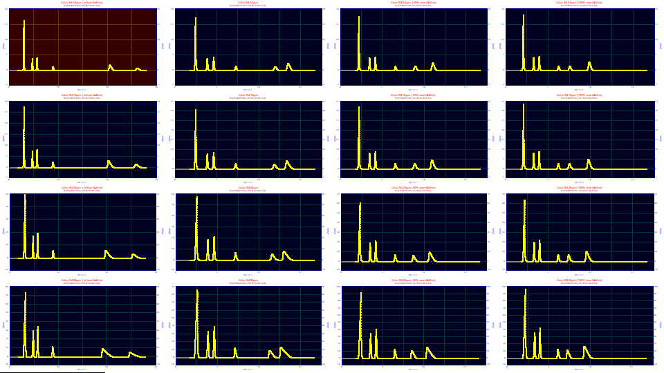
Click the Open button, the first button in the program's main toolbar. Select the file CationTutorial2.pfd from the program's installed default data directory (\PeakLab\Data).

Deconvolving a Fitted IRF

When a standard is accurately fitted with an IRF, those parameters can be used in the IRF Deconvolution procedure to remove that instrument/system response prior to fitting a closed form model. Although this is a two step process, it can be quite fast and once an IRF is known, it can be removed from any applicable data set. To effectively fit an IRF model, the peaks need to be baseline resolved and a convolution integral is fitted, which can be appreciably slower.

Click on the IRF Deconvolution button in the main window.

if you did the second tutorial, click the Import from Fit button. We will import averaged values from the fits saved in the second tutorial.

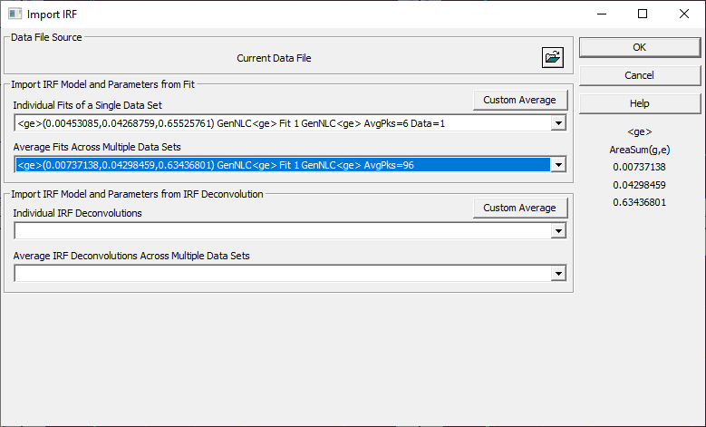
Select the <ge> fits in the Average Fits Across Multiple Data Sets dropdown. Click OK.

If you did not do the second tutorial, you will need to manually enter the three IRF parameter values as listed below.

Be sure the following values are set in the IRF Deconvolution dialog:

Response Fn
  <ge> AreaSum g,e
  Deconvolve Right
IRF Parameters
  0.0073714
  0.0429846
  0.6343680
Genetic Alg Optimization
  These settings will not be used
Fourier Filter
  D2 Automatic (the FFT threshold will be determined using a smoothed 2nd derivative)
  8 (8% smoothing for the D2 algorithm)
Post-Processing
  Zero Baseline Points - unchecked (baseline will be actual subtracted values)
  Zero Negative Points - unchecked (negative baseline points are permitted)

Click the Zoom-In Applies to All Graphs - X Scaling Only button in the toolbar of the graphs.

Use the mouse to zoom-in the first three peaks in the first graph.

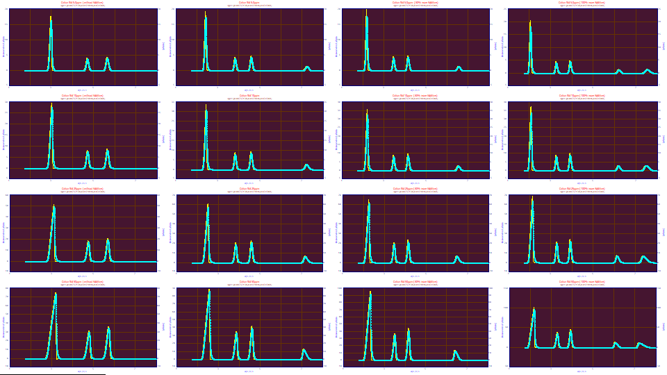
Viewed in this way, the averaging appears adequate. The deconvolutions look reasonable.

Click OK to exit the IRF Deconvolution procedure. Click OK to accept the default titles for this new data level in the data file containing this deconvolved data. The deconvolved data set is now selected in the main window.

Fitting the Data with the IRF Removed

We used Fourier deconvolution to remove the IRF from the data. We can now fit the fast closed form models to this deconvolved data. We assume the instrumental/system distortions have been mathematically removed.

Fitting the GenNLC Closed Form Model

Click the Local Maxima Peaks button in the main window to open the peak placement screen. Ensure the following settings are selected:

Peak Detection
  Set Sm n(1) to 25
Peak Type
  Select Chromatography in the first dropdown
  Select GenNLC as the model in the second dropdown
Scan
  Set the Amp % threshold to 1.5 %
  Leave Use Baseline Segments unchecked
  Be sure Use IRF,ZDD is checked
Vary
  Leave width a2 and shape a3 checked, all other unchecked

Click the Peak Fit button in the lower left of the dialog to open the fit strategy dialog. Select the Fit with Reduced Data Prefit, Cycle Peaks, 2 Pass, Lock Shared Parameters on Pass 1. Leave the Fit using Sequential Constraints box checked. Click OK.

As the fitting proceeds, you may wish to uncheck the Iteration Update. This updates each fit's graph with each successive improved iteration of that fit. Fits are faster without this graphical update.

Although we are not fitting an IRF, we are still fitting a higher order ZDD parameter. The 2-Pass option first estimates the main peak parameters while the starting estimate for the ZDD asymmetry is held constant. When multiple peaks are present, especially with a significant variation in amplitude, the Cycle Peaks option will individually fit peaks within the overall fit, enabling even small amplitude peaks to be accurately fitted.

The sixteen fits should require just a few seconds. All of the threads/cores of your CPU are simultaneously used to make this fitting as fast as possible.

Click Review Fit.

The GenNLC Fits with the IRF Pre-deconvolved Data

Click Numeric, and in the Options menu choose Select Only Fitted Parameters and check Average Multiple Fits. Scroll to the bottom of the Numeric Summary.

Average for 16 Fits

Fitted Parameters

r² Coef Det        DF Adj r²          Fit Std Err        F-value            ppm uVar

0.99995804         0.99995795         0.02531326         24,665,342         41.9592113

 Peak        Type                a₀                a₁                a₂                a₃                a₄    

    1        GenNLC        8.07479019        2.30934258        0.00027187        -0.0099375        1.04831845  

    2        GenNLC        2.25529475        3.77250138        0.00029195        -0.0016416        1.04831845  

    3        GenNLC        2.61961968        4.54344339        0.00027784        -0.0008759        1.04831845  

    4        GenNLC        1.18644131        7.22104750        0.00039602        0.00189999        1.04831845  

    5        GenNLC        2.52708365        12.3209593        0.00086309        0.01873860        1.04831845  

    6        GenNLC        3.58674858        15.2890117        0.00099722        0.02611136        1.04831845 

Note that the a₀ area and a₃ chromatographic distortion parameter averages mean little since these parameters are concentration dependent, and the data samples vary a full order of magnitude in concentration.

The goodness of fit values range from 9.80 - 131 ppm.

The second tutorial fitted these same sixteen data sets to a GenNLC<ge> model with an average goodness of fit of 10.3 ppm unaccounted variance, varying from 5.0 - 20.6 ppm:

Average for 16 Fits

Fitted Parameters

r² Coef Det        DF Adj r²          Fit Std Err        F-value            ppm uVar

0.99998974         0.99998972         0.01494899         58,763,437         10.2583889

 Peak        Type                    a₀                a₁                a₂                a₃                a₄                a₅                a₆                a₇    

    1        GenNLC<ge>        8.07933699        2.30784582        0.00026474        -0.0099790        1.11887780        0.00737138        0.04298459        0.63436801  

    2        GenNLC<ge>        2.25247000        3.77100711        0.00029000        -0.0016692        1.11887780        0.00737138        0.04298459        0.63436801  

    3        GenNLC<ge>        2.61798274        4.54185798        0.00027606        -0.0009040        1.11887780        0.00737138        0.04298459        0.63436801  

    4        GenNLC<ge>        1.18633675        7.21994862        0.00039513        0.00189375        1.11887780        0.00737138        0.04298459        0.63436801  

    5        GenNLC<ge>        2.52764231        12.3193707        0.00086418        0.01870488        1.11887780        0.00737138        0.04298459        0.63436801  

    6        GenNLC<ge>        3.58747556        15.2877892        0.00099840        0.02611155        1.11887780        0.00737138        0.04298459        0.63436801  

By preprocessing the data with the average IRF from the 16 fits, removing this average IRF from all 16 data sets using Fourier deconvolution, we see see an average error of 42 ppm. Since one is deconvolving an average IRF estimate on all data sets, where such was seen as having a some variability, and since deconvolution adds noise, we expect a weaker goodness of fit.

Click OK to close the Review window. Check Save updated information to the current data file when adding fits and click OK, accepting the default name for the fit. Click OK to confirm and click OK one last time to leave the placement screen and return to main screen.

An Alternative to IRF Determination by Convolution Fitting and Averaging

Averaging a number of IRF estimates from standards which are truly representative of the production samples will serve you well, provided you do not vary formula or settings which cause the IRF to vary from expectation, and assuming column health remains good.

PeakLab offers an alternative to convolution integral modeling for determining the IRF of real-world data for those instances where the peaks are baseline resolved, and the baseline is cleanly subtracted. In this instance, a genetic optimization is used to estimate the values of the IRF in an approach wholly distinct from the nonlinear convolution fitting.

This is especially attractive for the <pe> IRF, which is harder to fit in convolution models because the long tails of the 1.5 order kinetic component are more easily correlated with the slower exponential component at certain parameter guesses in the iterative fitting.

Change the Data Level to the entry that begins with 'BL', the baseline correction that was fitted. It will be second in the dropdown.

With the exception of the Section procedure, which does not actually modify the data (only the active and inactive state of the points), the different procedures in the program that alter the data values always process the uppermost level of data. To create an alternative convolution, we must not use the uppermost "DC" level we just created since this consists of data that has already seen this deconvolution. We must first create a copy of the baseline-corrected data we used for this first deconvolution.

Click the Copy button in the Data Levels portion of the dialog. Click Yes to confirm the copy of the 'BL' baseline-corrected level to the uppermost level and OK to accept the default data level name and the data titles for this level. These will be updated when this copied level becomes a second deconvolved data level.

Click on the IRF Deconvolution button in the main window. The values should be those we just entered so that we can visually explore this average across the different data sets. Here we will also specify the generic algorithm settings:

Response Fn
  <ge> AreaSum g,e
  Deconvolve Right
IRF Parameters
  0.0073714
  0.0429846
  0.6343680
Genetic Alg Optimization
  90% (Parameter 1) 0.0073714 ± 90%
  20% (Parameter 2) 0.0429846 ± 20%
  50% (Parameter 3) 0.6343680 ± 50%
  BsLnZero (we want to maximize the baseline points)
  0.50 % (the baseline region is defined as ±0.5% of the amplitude)
Fourier Filter
  D2 Automatic (the FFT threshold will be determined using a smoothed 2nd derivative)
  8 (8% smoothing for the D2 algorithm)
Post-Processing
  Zero Baseline Points - unchecked (baseline will be actual subtracted values)
  Zero Negative Points - unchecked (negative baseline points are permitted)

The Zoom-In Applies to All Graphs option in the toolbar of the graphs will be selected upon entry into the procedure. We will use this zoom-in to see a fixed zone of baseline in each graph.

Use the mouse to zoom-in the first three peaks in the first graph. Additionally zoom-in just the baseline region.

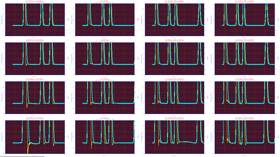
When the deconvolution using the average IRF from the convolution fits is strongly zoomed-in, it is apparent this averaged IRF is not at an optimum for most of the data sets. The concentration increases by rows: 5 ppm in the first row, 10 ppm in the second, 25 ppm in the third, and 50 ppm in the fourth. The additive increases by columns: 0x, 1x, 1.5x, and 2x. Looking at the additive trends across the four rows of graphs, we see we tend to be too strong in the deconvolution with no additive and too weak with 2x additive. With increasing concentration, we see mostly the scaling to a fixed y range. If you look very closely, you will probably find something to dislike visually with each of the 16 deconvolutions.

Click the Generic Optimize button.

The procedure is mathematically intensive, and will require perhaps minute to optimize all sixteen data sets. All cores and threads are used in the genetic algorithm, so the more capable your CPU, the faster the optimizations will be. These do require a random progression (a genetic differential evolution) and for each set of trial estimates a Fourier deconvolution must be performed and analyzed. When an optimization is complete, that data set will be graphed with the optimized deconvolution and the background color will change to indicate a custom parameter set (differing from the values set in the dialog).

The GA optimization is based on the premise that the settings which maximize the baseline represent the optimum deconvolution.

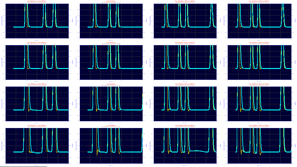
  When the optimizations are complete, click the List Parameter Estimates button.

IRF       Parm1            Parm2            Parm3            Data

<ge>      0.0007371      0.0443169      0.5909612      CationStd-5ppm-0x

<ge>      0.0007371      0.0458846      0.5739107      CationStd-5ppm-1x

<ge>      0.0007371      0.0465199      0.5716800      CationStd-5ppm-1.5x

<ge>      0.0007371      0.0462845      0.5623338      CationStd-5ppm-2x

<ge>      0.0007371      0.0428577      0.5727528      CationStd-10ppm-0x

<ge>      0.0007371      0.0452781      0.5869663      CationStd-10ppm-1x

<ge>      0.0007371      0.0452583      0.5698625      CationStd-10ppm-1.5x

<ge>      0.0007371      0.0465040      0.5797757      CationStd-10ppm-2x

<ge>      0.0007371      0.0420473      0.5726280      CationStd-25ppm-0x

<ge>      0.0007372      0.0436653      0.5739285      CationStd-25ppm-1x

<ge>      0.0011291      0.0447747      0.6163836      CationStd-25ppm-1.5x

<ge>      0.0007371      0.0450597      0.5760548      CationStd-25ppm-2x

<ge>      0.0007371      0.0399514      0.5532984      CationStd-50ppm-0x

<ge>      0.0009950      0.0422471      0.5861017      CationStd-50ppm-1x

<ge>      0.0008931      0.0445735      0.6028895      CationStd-50ppm-1.5x

<ge>      0.0007411      0.0445609      0.5772500      CationStd-50ppm-2x

Note that a genetic algorithm uses random values to arrive at its solution, and you may see results which slightly differ from the above IRF estimates. This kind of Fourier optimization problem, plagued by local minima, is ideally managed by a fast genetic algorithm.

When fitting a convolution model, each peak is a convolution integral and there must be limits on the lower bound of the half-Gaussian, the 'g' component in the <ge> IRF. On the other hand, when deconvolving the <ge> IRF, as is being done in this procedure, one is deconvolving the IRF from the entire data set, irrespective of the count of peaks present. For this GA optimized deconvolution, this narrow width lower bound in the IRF of convolution models is not imposed. You will thus note that every data set optimized to a very narrow half-Gaussian width (Parm1), some to the lower limit set in the GA % limits. This optimization confirms the narrow width component is significant, better than half the area of the IRF in every instance, but of so small a width it is almost an impulse. This is one explanation as to why the <ge>, <pe>, and <e2> IRFs can be used almost interchangeably. Note also the constancy in the higher width exponential (Parm 2) and the area fraction of the narrow component (Parm3).

Close the List window.

An Additional Optional Exercise

If you would like an interesting additional exploration at this point, select the <e2> or <pe> IRF and click the Genetic Optimize button. Despite significant differences in the narrow width component in the <ge>, <e2> and <pe> IRFs, the deconvolutions will look remarkably similar. You might also find it interesting to explore the single exponential, the <e> IRF, if you feel the narrow width component could perhaps be omitted. You will not be able to optimize the <e> IRF-every value of an <e> parameter produces a poorer merit function than the non-deconvolved data. You will have to manually enter a value similar to 0.03 for the <e> parameter to see why this is so. It is a lovely way to visually confirm the necessity of this narrow width component in a chromatographic IRF. If you explore any of these other IRFs, select and optimize the <ge> once again before continuing with this tutorial.

The GenNLC Fits with the GA Optimized IRF Pre-deconvolved Data

Note that we did not use an average IRF; each of the data sets had its own estimated IRF in the deconvolution.

Click OK to exit the IRF Deconvolution procedure, OK to acknowledge the local deconvolution notification (all are locally set if GA estimated), and OK to accept the default titles for this second deconvolved data level in the data file. This new deconvolved data level is now uppermost in the data file and it is also selected in the main window.

Click the Local Maxima Peaks button in the main window to open the peak placement screen. The prior settings are remembered. We will again be fitting the closed form GenNLC model.

Click the Peak Fit button in the lower left of the dialog to open the fit strategy dialog. Select the Fit with Reduced Data Prefit, Cycle Peaks, 2 Pass, Lock Shared Parameters on Pass 1. Leave the Fit using Sequential Constraints box checked. Click OK.

Click Review Fit.

Click Numeric, and in the Options menu choose Select Only Fitted Parameters and check Average Multiple Fits. Scroll to the bottom of the Numeric Summary.

Average for 16 Fits

Fitted Parameters

r² Coef Det        DF Adj r²          Fit Std Err        F-value            ppm uVar

0.99996768         0.99996761         0.02640061         23,900,180         32.3182938

 Peak        Type                a₀                a₁                a₂                a₃                a₄    

    1        GenNLC        8.07888262        2.31690150        0.00029312        -0.0097789        0.98443932  

    2        GenNLC        2.25586357        3.77827862        0.00029543        -0.0016222        0.98443932  

    3        GenNLC        2.62037724        4.54892853        0.00028019        -0.0008688        0.98443932  

    4        GenNLC        1.18691783        7.22571489        0.00039726        0.00188481        0.98443932  

    5        GenNLC        2.52745307        12.3255234        0.00086439        0.01872755        0.98443932  

    6        GenNLC        3.58716871        15.2936918        0.00099916        0.02611948        0.98443932  

By this GA optimization, we have reduced the average error across the 16 data sets from 42.0 ppm using an average of the IRFs from the convolution fits to 32.7 ppm. This is an improvement, but still nowhere close to the 10 ppm average error of the GenNLC<ge> convolution fits. The errors of fit across the 16 data sets range from 9.01 - 46.7 ppm, a significant improvement in the data sets least effectively fitted when using an average IRF from fitting convolution models.

Click OK to close the Review window. Click OK, accepting the default name for the fit. Click OK to confirm and click OK one last time to leave the placement screen and return to main screen.

Locking the Average IRF Values for Subsequent Fits

We will explore one further option in this tutorial. We know IRF deconvolution adds noise. An option to remove this impact is to fit the convolution models with the IRF parameters locked at the previously estimated averages. The fits will not be closed form, and thus slower because of the convolution integrals still being fitted, but the noise arising from the deconvolution will be absent.

Change the Data Level to the entry that begins with 'BL', the baseline correction that was fitted.

Click the Local Maxima Peaks button in the main window to open the peak placement screen. The prior settings are remembered. We will again be fitting the closed form GenNLC model.

Click the IRF button and enter 0.0073714, 0.0429846, 0.6343680, our averages for the <ge> parameters, in the <ge> section in this dialog (upper left). Also click the Lock buttons on all three parameters. Click OK.

Select the GenNLC<ge> model. Click the Peak Fit button in the lower left of the dialog to open the fit strategy dialog. Select the Fit with Reduced Data Prefit, Cycle Peaks, 2 Pass, Lock Shared Parameters on Pass 1. Leave the Fit using Sequential Constraints box checked. Click OK.

After the fitting is complete. click Review Fit.

Click Numeric, and in the Options menu choose Select Only Fitted Parameters and check Average Multiple Fits. Scroll to the bottom of the Numeric Summary.

Average for 16 Fits

Fitted Parameters

r² Coef Det        DF Adj r²          Fit Std Err        F-value            ppm uVar

0.99997735         0.99997730         0.01898578         37,488,984         22.6508064

 Peak        Type                    a₀                a₁                a₂                a₃                a₄                a₅                a₆                a₇    

    1        GenNLC<ge>        8.08594987        2.30807271        0.00026604        -0.0099521        1.09407482        0.00737140        0.04298460        0.63436800  

    2        GenNLC<ge>        2.25705595        3.77110554        0.00028976        -0.0016624        1.09407482        0.00737140        0.04298460        0.63436800  

    3        GenNLC<ge>        2.62101056        4.54191884        0.00027588        -0.0008993        1.09407482        0.00737140        0.04298460        0.63436800  

    4        GenNLC<ge>        1.18734441        7.22006712        0.00039529        0.00189655        1.09407482        0.00737140        0.04298460        0.63436800  

    5        GenNLC<ge>        2.52765222        12.3199427        0.00086380        0.01875207        1.09407482        0.00737140        0.04298460        0.63436800  

    6        GenNLC<ge>        3.58746198        15.2882163        0.00099839        0.02616161        1.09407482        0.00737140        0.04298460        0.63436800  

We now have a basis for estimating the analytical cost of using Fourier deconvolution in a preprocessing step followed by a very fast closed-form fitting. The error with locked estimates of the IRF on the convolution models averages 22.6 ppm across the sixteen data sets. The error with the Fourier deconvolution and closed form fits was 41.9 ppm. If we compare the a₂-a₄ higher moment parameter averages, the differences are modest. If you want the minimum of noise in your fits, and fitting time is not an issue for you, this approach of locking the known IRF in convolution model fits is recommended. Here we repeat the fit averages for the deconvolved data.

To summarize the average goodness of fit for the sixteen data sets:
     Full GenNLC<ge> convolution model = 10.25 ppm
     GenNLC<ge> with locked <ge> average IRF = 22.65 ppm
     Fourier deconvolution using individual estimates of IRF, fitted by GenNLC = 32.32 ppm
     Fourier deconvolution using fitted IRF average, fitted by GenNLC = 41.96 ppm

We can assume the additional unaccounted variance arising from using an averaged IRF is about a doubling, and that the noise introduced in the Fourier deconvolution adds approximately another doubling.

Click OK to close the Review window. Click OK, accepting the default name for the fit. Click OK to confirm.

Click the IRF button and remove the Lock on the three <ge> parameters previously set. The IRF and ZDD customizations are global and remain in place until changed. Click OK.

Click OK one last time to leave the placement screen and return to main screen.

Fitting an IRF Convolution Model vs Deconvolving the IRF and Fitting a Closed-Form Model

Fitting an IRF-bearing convolution model, such as the GenNLC<ge> (as we fit above with locked parameters) is not the same analytical process as employing a Fourier deconvolution to remove the <ge> IRF and then subsequently fitting a closed form GenNLC model. For one, only convolution occurs in the first instance, and only deconvolution in the second. The convolution process smoothes data, the deconvolution process adds noise. That noise is usually filtered within the Fourier domain during the inverse which follows the deconvolution, but that noise filtering may add its own bias. The results of both approaches will be quite close, but there will be differences, especially in the higher moments.

Convolution vs. Deconvolution

If you need the most accurate a₃ chromatographic distortion and a₄ asymmetry parameters possible, you will probably want to fit the convolution integral directly. If you do not have baseline resolved peaks with at least one of the peaks intrinsically fronted, you may need lock an average IRF as we did in the last example. Otherwise, you should be able to use either of the approaches illustrated in this tutorial for a Fourier deconvolution preprocessing step followed by a very fast and efficient closed form model fit. We observed that the two-step process, despite using exactly the same IRF parameter values, adds the noise from the Fourier deconvolution that was not filtered, as well as any bias arising from this signal filtration.

In discrete Fourier processing, convolution and deconvolution will have subtle differences. When we fit a convolution integral, such as the GenNLC<ge>, we fit a convolution. The different tiers of deconvolution are parametric and derived from the fitting; one can generate an IRF-free GenNLC by using the a₀-a₄ parameters of the GenNLC<ge> fit, or an IRF-free and ZDD-free NLC by using the a₀-a₃ parameters, or even an infinite dilution Giddings peak using the a₀-a₂ parameters. In an <irf> fit, there is no Fourier deconvolution, only Fourier convolution. All deconvolution is parametric, and noise free.

However elegant and efficient from a goodness of fit perspective, there are significant drawbacks to a convolution model fit where the IRF is estimated. The data must be clean enough to expose the IRF for such estimation, meaning at least certain peaks must be baseline resolved and ideally with one or more intrinsically fronted (-a₃) peaks to help statistically separate a₃ from a₄. Because of multiple parameters which can compete in addressing tailing, the S/N must be strong. The fits may not be possible if only intrinsically tailed peaks are present in the data. Also, convolution models are integrals computed in Fourier domain convolutions, and thus much slower to fit than closed form models.

The main benefit of a convolution model fit is that every fit will contain parameters that give you estimates of system stability and column health to the extent the IRF parameters are accurately estimated. The goodness of fit is also potentially higher.

Deconvolution vs Convolution

Deconvolution is fast, efficient, and once an IRF for a given instrument, column, and prep is quantified, it can be used to render any data set amenable to closed form model fits. Data which have overlapping and hidden peaks aren't an issue, and with an automated filter, such as the D2 filter we used in this tutorial, varying S/N can often be transparently managed. This two-step approach works whether or not the peaks are baseline resolved, no matter how messy the data happens to be. Closed-form fits are also far less susceptible to failed fits arising from correlated parameters since no IRF is fitted. They are also exceptionally fast, usually mere seconds or less for multiple high sampling-density data sets.

There are drawbacks to deconvolution followed by a closed-form model fit. The IRF must first be predetermined by some method, either fitting a convolution model or by a genetic optimization of the deconvolution. The goodness of fit will definitely be weaker as a consequence of the noise introduced by discrete deconvolution, and unless each data set is independently optimized with the genetic algorithm, there will be a small diminishing of the goodness of fit by the imposition of an averaged IRF estimate.

In Perspective

To put these differences in perspective, the best fit realizable in prior releases of the technology, the NLC, generated an 3470 ppm average error for these sixteen fits. In the above discussion, we address average errors which range from about 10 - 40 ppm. The reason we give such attention to this refinement in fitting is that the higher moments and the IRF parameters are important in measuring system stability and performance, and in any process optimization. If you wish to know if small changes in formulations produce better separations, you need to know if a change increases or diminishes the IRF distortions and the deviations from ideality represented in the higher moment parameters.

For most analytical work, identifying the IRF for a given column's general procedure and using IRF Deconvolution followed by closed-form GenNLC or GenHVL fits may be all you ever need. As a crosscheck on system stability, however, we would recommend routine convolution fits for the standards to ensure there have been no changes in the system or column health.