PeakLab v2 Documentation Contents R2N Software Home R2N Software Support
Delta-Impulse/Density Chromatographic Models
Nonlinear Chromatography
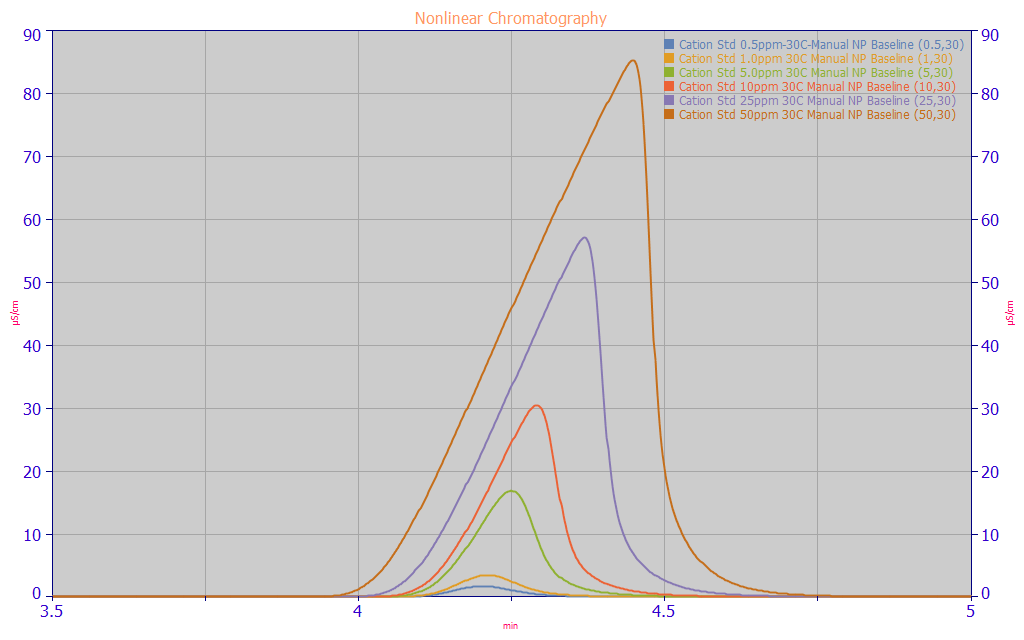
Nonlinear chromatography is seen when the concentration of a chromatographic analyte increases, and there is an increase in the peak's 'tailing' or 'fronting'.

In the above plot a Lithium peak in cation IC chromatography is shown with concentrations that vary two orders of magnitude from 0.5 ug/ml to 50 ug/ml. This peak, which is nearly symmetric at very low concentrations, becomes sharply 'fronted' at much higher concentrations. The change in the characteristic tailing or fronting of chromatographic peaks with concentration is quantified in a chromatographic model by a parameter known as the distortion, chromatographic distortion, or fronting-tailing factor. In PeakLab, the chromatographic distortion arising from the nonlinearity of concentration dependence is always parameter a3 in the delta-impulse/density models in the program.
Linear Chromatography

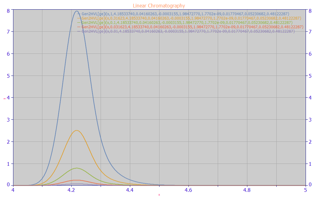
When the chromatographic peak shape is constant, there is a linear increase in the signal at every point from an increased concentration. In the above plot, the shape from the amber peak in the first plot is maintained through two orders of magnitude lower concentration. In our experience, a linear regime of chromatographic separation doesn't imply that the delta-impulse/density nonlinear models are invalid, only that this concentration dependence is too small to be visually observed in plots of the peaks.
The HVL Chromatographic Model
The Haarhoff-Van der Linde or HVL model is far and away the best known Delta-Impulse/Density model. In these models the differential equations which assume a given density for the peak broadening from the separation are solved for a delta-input injection. The HVL produces the type of concentration dependence shown in the first plot for an 'infinite dilution' or 'zero distortion' density which is Gaussian. In PeakLab, this core density in this type of delta-input/density model is referred to as the 'ZDD', the zero-distortion density. it is the density you would see as the concentration is reduced to where the peak is only barely able to be detected.
The HVL model assumes a theoretical Gaussian diffusion. Since the normal is the simplest density, the HVL can be seen as the simplest of the delta-input/density chromatographic models. It is defined as follows:
(1)
If we look at the HVL as a statistical model absent its theoretical derivations, and in a form where the area is an adjustable parameter, we have a four parameter function. In this form, a0 is the peak area, a1 is the center or location value, a2 is the peak width or scale parameter, and a3 is the shape parameter, positive for a right-skewed asymmetry, negative for left-skewed. In the HVL, a1 is the mean-mode-median of the underlying Gaussian zero-distortion density, not the mode or location of the apex of the peak.
The HVL Chromatographic Generalization
In order to generalize the HVL model, we use the Gaussian or normal probability density function (PDF), normalized to unit area:
(4)
We also use the Gaussian or normal cumulative distribution function (CDF):
(5)
We can now rewrite the HVL as a generalized delta-input/density template that accepts any zero-distortion density:
(7)
To regenerate the HVL, Density is replaced with (4), the normal PDF, and Cumulative with (5), the normal CDF.
The NLC Chromatographic Model
The Wade-Thomas NLC (nonlinear chromatography) model was originally derived to model the kinetics in liquid ion-chromatography (IC) separations. The same delta impulse input is assumed in the solution of the differential equations, but the density assumed will be the Giddings model which describes the peak shape that is seen as the concentration approaches an infinite dilution. The Giddings peak is a kinetic model that requires a retention scale in order for the kinetic broadening parameter to have theoretical meaning. Although the NLC was designed for slow adsorption-desorption kinetics, it has shown itself to be versatile where any form of mass transfer resistance can be modeled with first order kinetics.
Although the NLC model is very difficult to implement (modified Bessel functions and modified Bessel function integrals), it would often prove to be the most effective of the original PeakFit chromatographic models in most HPLC and UHPLC separations.
The Wade-Thomas NLC model is defined as follows:
(2)
Where TFn is a Bessel function integral:
(3)
When the area is an adjustable parameter, the NLC is also a four parameter function. As with the HVL, a0 is the peak area and a1 is the center or location value, and a3 is the distortion parameter, positive for the right-skewed asymmetry of a tailed peak and negative for the left-skewed asymmetry of a fronted peak.
This PeakLab NLC parameterization uses a time constant instead of a rate constant for the a2 kinetic parameter given in the original publication of the Wade-Thomas NLC model. As such, the NLC a2 is similar to the HVL a2, a scale parameter that increases with the peak width.
The NLC Chromatographic Generalization
To create a generalized NLC model template, we use the Giddings probability density function (PDF):
(8)
We also use the Giddings reverse cumulative or cumulative distribution function complement (CDFc):
(10)
The NLC density generalized template can then be expressed as follows:
(11)
Just as with the HVL template, we can create any number of NLC generalized models by inserting a matched density-cumulative pair other than the Giddings for the zero-distortion assumption.
To regenerate the NLC, Density is replaced with (8), the Giddings PDF, and RevCumulative with (10), the Giddings CDF complement.
The Common Distortion Model
Although one of these templates uses a CDF and the other a CDF complement, the templates can produce identical shapes for a given density-cumulative pair. One can substitute the Gaussian density in the NLC template to generate the HVL shapes, and the Giddings density can be inserted into the HVL template to produce the NLC shapes. The main differences rest in the two templates rests with the parameterization of a3. In the HVL, a3 is scaled by a2/a1, common with statistical densities, whereas the kinetics of the NLC model directly scale with time.
These two templates are used interchangeably within PeakLab, where possible, to construct models with a maximum dynamic range of a3 chromatographic distortions.
Note that the a1 associated with the first moment, and the a2 associated with the second moment also appear in the templates, and while the a1 center values are comparable, the a2's consist of immensely different representations of the peak widths, one a Gaussian diffusion width, the other a kinetic time constant associated with adsorption-desorption.
Because the generalized HVL (GenHVL) and generalized NLC (GenNLC) models can produce exactly the same shapes, it is possible to convert a fitted a2 so that it represents either an HVL diffusion width or an NLC kinetic time constant. This is what is given in the Equivalent Parameters section of the Numeric Summary of a fit.
Densities with an Adjustable Third Moment Term
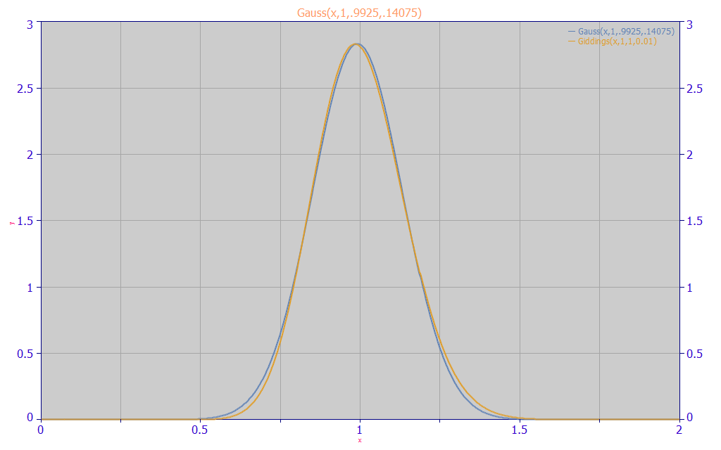
The major drawback of the HVL and NLC models is that the higher moments are fixed by the Gaussian and Giddings zero-distortion assumptions. Despite the fact the HVL and NLC were derived at very different times for GC and IC, the HVL and NLC models have always generated very similar peak shapes and similar goodness of fit values. This can be attributed to the similarity between the Gaussian and Giddings zero-distortion densities:

The Giddings density, the amber curve, is a slightly right-asymmetric peak as compared to the symmetric Gaussian, the blue curve. This symmetry explains why the HVL produces mirrored shapes about a1 when reversing the sign of a3, whereas the NLC produces different tailed and fronted shapes on each side of a1 with reversed signs of a3.
In our experience, it is rare that either the HVL or the NLC will precisely fit a given chromatographic peak. In general, there will be some measure of third moment asymmetry (skewness) in the underlying zero distortion density. In HPLC and UHPLC, the pore density of the particles may not be perfectly symmetric, or the column packing may be less than ideal, or other real-world nonidealities may exist within the actual separation. For example, with the NLC kinetics, a single site adsoprtion-desorption is assumed.
Although for many HPLC and UHPLC peaks, the asymmetry of the NLC with the slightly right-skewed Giddings will offer improved fits with respect to the HVL, it is worth noting that the NLC is a pure kinetic model, and unless the a2 kinetic time constant is shared across all peaks in an analysis, each peak's concentration-independent asymmetry will vary with an independently fitted kinetic time constant. One advantage of kinetic models is that this a2 time constant can be assumed constant across all peaks eluting across time within a given chromatogram. In isocratic separations, peaks typically broaden with time. The kinetic models will estimate this broadening with time, but this will only work when first order kinetics apply.
The HVL and NLC generalized templates allow for any density-cumulative pair to be used to created generalized chromatographic models. In order to deal with the non-idealities in the actual chromatographic separation, we assume the ZDD is neither Gaussian (HVL) or Giddings (NLC) but is instead a more complex density that allows for the third moment, the skew to be broadly adjustable. This is the premise of most of the ZDD models in PeakLab.
The Delta-Impulse/Density models are a family of chromatographic models where this delta-input assumption is central to the model. In general, these chromatographic models will be specific to chromatography as a consequence of this injection pulse. You can think of the delta-impulse mathematics as a simple transform that introduces the concentration nonlinearity into a given density. Any density can be so transformed. The Gaussian density of the HVL represents the simplest of the statistical densities, and the Giddings density, the simplest of the kinetic densities. The following zero distortion densities are used in PeakLab to extend the modeling power of the Gaussian ZDD (HVL) and the Giddings ZDD (NLC) where a third moment is adjustable in the core zero distortion density:
Default Asymmetric Normal (GenHVL, GenNLC)
[Z] Asymmetric Normal (GenHVL[Z], GenNLC[Z])
[G] Half-Gaussian Modified Gaussian (GMG) (GenHVL[G])
[E] Exponentially-Modified Gaussian (EMG) (GenHVL[E])
[T] Generalized Student's t (Asymmetric) (GenHVL[T], GenNLC[T])
[V] Generalized GMG (GenHVL[V], GenNLC[V])
Densities with an Adjustable Fourth Moment Term
A fourth moment is essential for gradient and overload peaks, and it has also proven useful for detecting columns with less than ideal packing and for flagging peaks that have experienced some measure of detector saturation. These zero distortion densities add a fourth moment (kurtosis or fat tails) term:
Default Asymmetric Error Model (Gen2HVL, Gen2NLC)
[Y] Asymmetric Error Model (GenHVL[Y], GenNLC[Y])
[Q] Error Model (Symmetric) (GenHVL[Q])
[S] Student's t (Symmetric) (GenHVL[S])
[Yp] Generalized Error Model (High Overload Shapes Only) (GenHVL[Yp])
[YpE] Generalized
Laplace (High Overload Shapes Only) (GenHVL[YpE])
[Yp2]
Generalized Error 2-Width (Overload Shapes) (GenHVL[Yp2])
[Yp2E] Generalized Laplace 2-Width (High Overload Shapes Only) (GenHVL[Yp2E])
[K] Generalized Two-Sided Kinetic Orders 0,1 (High Overload Shapes Only) (GenHVL[K])
[W] Generalized Error, Linear Gradient (HPLC Gradient Peaks Only) (GenHVL[W])