PeakLab v1 Documentation Contents AIST Software Home AIST Software Support
HPLC Gradient Peaks - Direct Closed Form Fits (Tutorial)
In this tutorial, we will fit HPLC gradient peak data to good modeling accuracy by fitting closed form models that directly fit the shape of the resultant gradient peaks.
For fitting the peaks which occur during isocratic starts and holds, and for having a reference point, we will begin with quantifying the IRF that is present absent the gradient in this type of reversed-phase ultra HPLC.
Fitting Isocratic Peaks and the IRF Determination
We can estimate the system/instrument IRF using a peak that occurs during the isocratic start, where the mobile phase is not yet varying.
![]() Use the File menu's Open item and select the file HPLCGradientStd01.pfd from the
program's installed default data directory (\PeakLabv\Data). The file contains only a single data
set.
Use the File menu's Open item and select the file HPLCGradientStd01.pfd from the
program's installed default data directory (\PeakLabv\Data). The file contains only a single data
set.
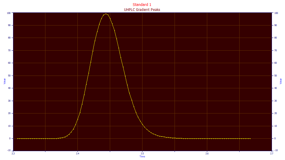
This baseline-corrected peak was from the starting portion of the elution where the mobile phase was constant. The peak appears to be slightly tailed, but this is one more instance where the true peak absent the instrumental/system distortions is intrinsically fronted and appears tailed only because of the presence of the IRF. Even though the sample concentrations in this type of gradient HPLC are very low, the instrumental/system distortions still exist, and as a first step we will quantify an IRF describing these.
We will fit a two component IRF, one with both a 'fast' and 'slow' component. Here we will introduce a couple of factors of experience. After a large number of data fits, our experience suggests the IRFs for nearly all chromatographic peaks have such a fast and slow component, and that in general, the slower component will be an 'instrument' distortion that is independent of most process variables and is almost perfectly modeled by a first order exponential, and the faster component will be a 'system' distortion will will be sensitive to system variables such as sample concentration, temperature, additive levels, etc. and where the model is less clear since it has much less influence on the peak tailing. We further note our experience which suggests the faster component tends to comprise about 5/8 of the overall area in a composite or two-component IRF model.
Although the gradient compresses any tailing arising from an IRF, possibly rendering both components unrecoverable in any mathematical process of unwinding the compression, we are at this point only interested in accurately estimating the isocratic IRF as best we can. Such will definitely be applicable to peaks occurring in the holds where the mobile phase is not varying.
We will use the <ge> model for the IRF, locking the 5/8 half-Gaussian area fraction in order to ensure the narrow width component does not iterate to near zero widths or area fractions. Our focus here will be the more prominent exponential time constant, since it is this component of the IRF that is most likely to have a portion survive the gradient compression and thus have an influence on the final gradient peak shape.
In this instance we will use a GenHVL (generalized HVL) peak model for the chromatographic peak since it furnishes a statistical deconvolved Gaussian SD width for the peaks.
Fitting the GenHVL<ge> Model
Click the Local Maxima Peaks button in the main window to open the peak placement screen. Ensure the following settings are selected:
Peak Detection
Set Sm
n(1) to 5
Peak Type
Select Chromatography
in the first dropdown
Select GenHVL<ge> as the model in the
second dropdown
Scan
Set the Amp %
threshold to 1.5 %
Leave Use Baseline Segments unchecked
Be sure Use IRF,ZDD is checked
Vary
Leave width a2
and shape a3 checked, all other unchecked
Click the IRF button and for the <ge> IRF, enter the following starting estimates: 0.01 for the g width (sd), .02 for the e width (tau), and .625 for the g area fraction. Click the Lock button for the g area fraction. Click OK. This type of chromatography will, in general, have smaller IRF widths than the program's defaults which are derived from fits of high S/N IC peaks.
Click the Peak Fit button in the lower left of the dialog to open the fit strategy dialog. Select the Fit with Reduced Data Prefit, 2 Pass, Lock Shared Parameters on Pass 1. Leave the Fit using Sequential Constraints box checked. Click OK. If you are fitting any peak model bearing IRF or ZDD parameter(s), you will almost always wish to use a 2-Pass option where the main peak parameters are first estimated while the starting estimates for the IRF and/or ZDD are held constant.
Even if each iteration where an improvement is realized is graphically updated, and even though an integral is being fitted, you should see a converged fit executed in less than a second. Click Review Fit. You should see a fitted peak with an unaccounted variance of just 5.17 ppm. This corresponds with an r2 coefficient of determination of .999995, a successful fit.
The lower graph, by default, shows only the fitted curve, the As Fitted selection in the first dropdown. There are additional dropdowns where you can see different aspects of the fitted peak. Select the IRF Deconv. option in the second dropdown. This plots, in the first aux component color (red by default for most color schemes), the fitted peak with the IRF removed, the GenHVL, the peak you would see if there existed no system/instrumental distortion. The IRF attenuates the peak and changes the shape, producing a stronger right skew.
Change the third dropdown to Partial Deconv. The second auxiliary component color is usually green by default. For this model, the green peak (the partial deconvolution) is the pure HVL, the theoretical peak after the ZDD's third moment non-idealities are mathematically removed. The red curve remains the peak absent the system/instrumental effects. Here you note that the difference,although modest, is one of a fronted peak, the HVL in green, versus that of a tailed peak, the generalized HVL, the GenHVL model, in red.
Change the fourth dropdown to Full Deconv. The third auxiliary component color is usually blue by default. For this model, the blue peak (the full deconvolution) is the pure Gaussian, the peak that would exist at infinite dilution. Despite the low concentrations, the a3 intrinsic chromatographic distortion changes the peak shape from the infinite dilution blue peak, to the fronted HVL peak in green.
![]() Click the Hide Y2 plot in the graph's toolbar. Use the mouse to zoom in just the peak.
Click the Hide Y2 plot in the graph's toolbar. Use the mouse to zoom in just the peak.
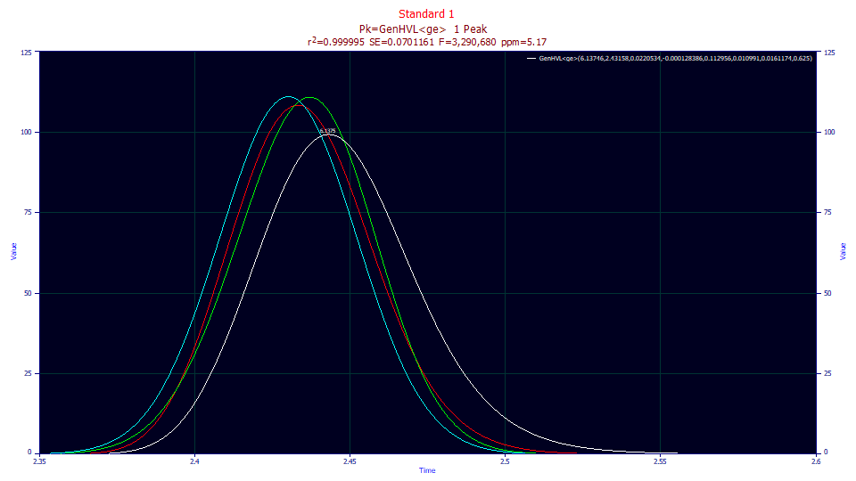
The white curve is the GenHVL<ge> peak fitted to the data registered by the instrument. The red curve is the GenHVL peak that would be seen if no IRF existed. The green curve is the fronted HVL that would be observed if the infinite dilution peak were a perfect Gaussian. The blue curve is that perfect Gaussian.
Change the second and third dropdowns to No Reference. This is the difference between the peak the instrument registered and what a pure infinite dilution peak would look like absent all instrumental/system distortions, all higher moment adjustments to the theoretical zero-distortion density, and all intrinsic chromatographic distortion.
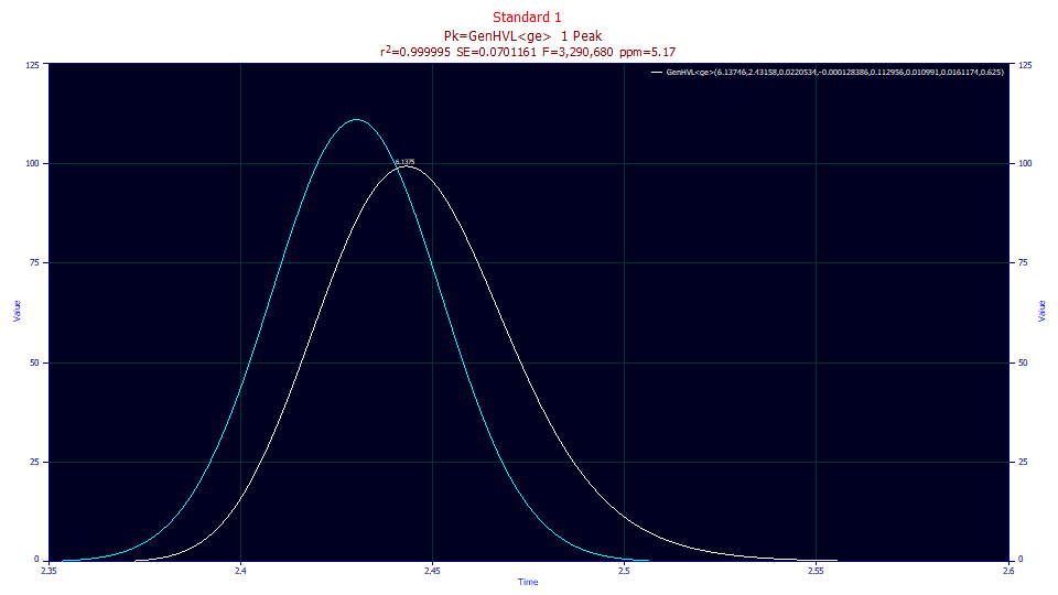
Click on the Numeric button to open the numeric summary. Under Options menu, choose Select All. To understand the full power of deconvolution, we will reference the moments in this numeric report.
Fitted�Parameters
r2�Coef�Det�� DF�Adj�r2���� Fit�Std�Err�� F-value������ ppm�uVar
0.99999483��� 0.99999448��� 0.07011614��� 3,290,680���� 5.16607737
�Peak�� Type�������� ������a0���� ������a1���� ������a2���� ������a3���� ������a4���� ������a5���� ������a6���� ������a7����
����1�� GenHVL<ge>�� 6.13746193�� 2.43158324�� 0.02205342�� -0.0001284�� 0.11295617�� 0.01099098�� 0.01611737�� 0.62500000��
Equivalent�Parameters
�Peak�� Type�������� ������a0���� ������a1���� ������a2���� ������a3���� ������a4���� ������a5���� ������a6���� ������a7����
����1�� GenNLC<ge>�� 6.13746193�� 2.43158324�� 0.00010001�� -0.0001284�� 12.4544071�� 0.01099098�� 0.01611737�� 0.62500000��
Measured�Values
�Peak�� Type�������� �Amplitude�� ��Center���� ���FWHM����� ��Asym50���� �FW�Base���� ��Asym10����
����1�� GenHVL<ge>�� 99.2921196�� 2.44334981�� 0.05751218�� 1.09098420�� 0.11698820�� 1.23178641��
�Peak�� Type�������� ���Area����� ��%�Area���� ���Mean����� ��StdDev���� �Skewness��� �Kurtosis���
����1�� GenHVL<ge>�� 6.13745695�� 100.000000�� 2.44708354�� 0.02554769�� 0.44089004�� 3.64278939��
Analytic�Moments
�Peak�� Type�������� ��FnArea���� �%�FnArea��� ��FnMean���� �FnStdDev��� FnSkewness�� FnKurtosis��
����1�� GenNorm[m]�� 6.13746193�� 100.000000�� 2.43158324�� 0.02226555�� 0.34140739�� 3.20793949��
Deconvolved�Moments
�Peak�� Type���� ���Area����� ���Mean����� ��StdDev���� �Skewness��� �Kurtosis��� �Amplitude�� ���Center�����
����1�� GenHVL�� 6.13746193�� 2.43563811�� 0.02266643�� 0.24913813�� 3.11566300�� 108.394890�� 2.43346960��
�Peak�� Type���� ���Area����� ���Mean����� ��StdDev���� �Skewness��� �Kurtosis��� �Amplitude�� ���Center�����
����1�� HVL����� 6.13746189�� 2.43556926�� 0.02210910�� -0.0899820�� 3.00242082�� 110.854630�� 2.43722184��
�Peak�� Type���� ���Area����� ���Mean����� ��StdDev���� �Skewness��� �Kurtosis���
����1�� Gauss��� 6.13746187�� 2.43033372�� 0.02205342�� 1.8039e-6��� 2.99999055��
Advanced�Area�Analysis
�Peak�� Type�������� ����Area���� ��%�Area���� �ApexAsym��� �NonOverlap1 ��%�PkArea�� �NonOverlap2 ��%�PkArea��
����1�� GenHVL<ge>�� 6.13745695�� 100.000000�� 1.15854123�� 0.26425149�� 4.30555353�� 1.11857651�� 18.2254071��
Parameter�Statistics
Peak�1�GenHVL<ge>
�Parameter����� Value������� Std�Error��� t-value����� 95%�Conf�Lo�� 95%�Conf�Hi�� P>|t|
���������Area�� 6.13746193�� 0.00180980�� 3391.23903�� 6.13387220��� 6.14105166��� 0.00000
�������Center�� 2.43158324�� 0.00175517�� 1385.38425�� 2.42810187��� 2.43506461��� 0.00000
��������Width�� 0.02205342�� 0.00036999�� 59.6059550�� 0.02131956��� 0.02278729��� 0.00000
�����Distortn�� -0.0001284�� 6.9666e-6��� -18.428657�� -0.0001422��� -0.0001146��� 0.00000
�������Z-Asym�� 0.11295617�� 0.00257834�� 43.8096003�� 0.10784204��� 0.11807030��� 0.00000
���������g-sd�� 0.01099098�� 0.00261730�� 4.19936324�� 0.00579958��� 0.01618238��� 0.00006
��������e-tau�� 0.01611737�� 0.00072271�� 22.3012528�� 0.01468388��� 0.01755087��� 0.00000
�������g-frac�� 0.62500000�� ������������ ������������ ������������� ������������� �������
Chromatographic�Analysis
�Peak�� Type�������� ��Nmoment��� ��Ngauss��� �FW�Base���� ��Asym10���� Resolution�� �Retention��
����1�� GenHVL<ge>�� 9174.74859�� 10008.4577�� 0.11698820�� 1.23178641�� ������������ 2.43158324��
In the Measured Values section are the moments for the actual peak as registered by the instrument. In the Deconvolved Moments section are the three peaks we visualized in the graphs. There is also a fourth deconvolution in the Analytic Moments section, the zero-distortion peak, the ZDD, the infinite dilution peak with the higher moment deviations from theoretical ideality included.
If we look at the progression, we go from a statistical skew of .441 from the peak as registered by the instrument, to .249 with the system/instrument response function removed, to -.090 for the theoretical HVL. There are two infinite dilution skews, the one actually produced by the generalized chromatographic peak, 0.341, and the 0.0 skew of the Gaussian.
The kurtosis, the fourth moment fatness of the tails, is 3.64 for the peak as registered by the instrument. When the IRF is removed, the GenHVL has a kurtosis of 3.12. Most of the excess kurtosis (statisticians speak of excess kurtosis as that which is above the 3.0 of the normal or Gaussian density) rests with the IRF. When the ZDD, the zero distortion density non-ideality fitting in the a4 skew term is removed or deconvolved, the pure HVL remains. Its kurtosis is very close to the Gaussian's 3.0.
The Advanced Area section offers an area asymmetry, the area to the right of the apex divided the area to the left. It also offers two measures of the convolution differences. The first is the measure of non-overlap between the theoretical peak and the generalized peak with the higher moments accounted, both of the peaks absent the IRF (the green and red curves above). In this example, 4.3% of the theoretical peak area fails to overlap the area in the generalized model, a measure of deviation from this theoretical expectation. The second overlap measures the difference between the generalized peak without the IRF and the full fitted model, the generalized peak with the IRF (the white and red curves above). Here the lack of overlap is 18.2%. Those two values answer indirectly how important the ZDD and IRF are in altering the shape of the observed peak. In our experience, the greater effect will usually rest with the IRF.
For the purposes of this example, we will merely note a system/instrument <ge> IRF whose tau or time constant width is 0.0161. We also note an a4 ZDD statistical asymmetry of .114. This varies from -1 to 1. A pure HVL peak maps to a symmetric Gaussian ZDD (a4=0). For this data, the real-world infinite dilution density is far from Gaussian.
The Parameter Statistics show this fit as statistically significant in all parameters (the values are grayed where this is not true). Note the 95% confidence limits for the exponential width as 0.0147 - 0.0176.
It is important to note that all three distortion effects continue to exist and are quantifiable in this non-gradient reversed-phase ultra-HPLC peak. The system/instrument effects alter the peak shape, the zero-distortion higher moment idealities remain significant, and the intrinsic chromatographic distortion must equally be treated as non-negligible. Each of these principal effects are significant if you wish to model any one of these deconvolutions as representative of your true peak, or if you wish to accurately characterize the system/instrumental effects, the higher moment deviations from non-ideality, or the concentration-dependent intrinsic distortion, as a measure of instrument/column health or performance.
Change the third dropdown back to No Reference. Click OK to close the Review. Check Save updated information to the current data file when adding fits and click OK, accepting the default name for the fit. Click OK to confirm and click OK one last time to leave the placement screen and return to main screen.
A Second IRF Estimation using a Genetic Algorithm Optimization of the IRF Deconvolution
Before we proceed to fitting the gradient peaks, we will explore a separate method for estimation of the isocratic IRF. In the prior section, we estimated the <ge> IRF parameter by fitting a GenHVL<ge> convolution model to a non-gradient peak. In this step, we will use the genetic algorithm built into the IRF Deconvolution procedure to directly estimate this parameter from the shape of the deconvolution. This genetic algorithm optimization relies on the observation that the optimal IRF parameters maximize the count and accuracy of baseline points.
Click on the IRF Deconvolution button and ensure the following settings are selected:
Response Fn
<e>
Exponential
Deconvolve Right
IRF Parameters
0.015
Genetic Alg Optimization
90 % (the 'g' half-Gaussian will vary from 0.015 to 0.0285)
BsLnZero (we want to maximize the baseline points)
0.50 % (the baseline region is defined as �0.5% of the amplitude)
Fourier Filter
D2 Automatic (the FFT threshold will be determined
using a smoothed 2nd derivative)
8 (8% smoothing for the D2 algorithm)
Post-Processing
Zero Baseline Points - unchecked (baseline will be
actual subtracted values)
Zero Negative Points - unchecked (negative
baseline points are permitted)
Click the Genetic Optimize button.
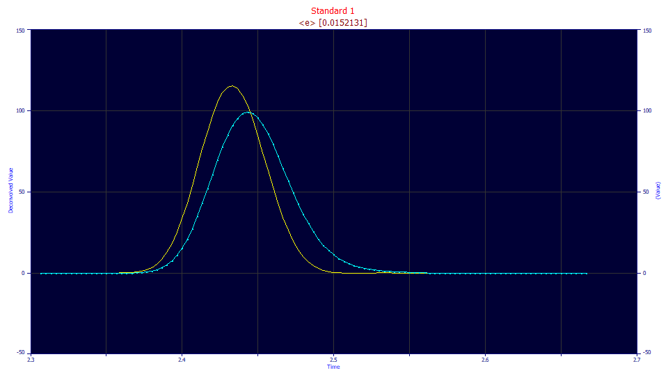
The genetic algorithm optimization estimates the optimum <e> exponential tau at 0.0152, close to the 0.0162 of the fitting procedure.
For the purpose of accurately fitting the isocratic peaks, we will use the values for two-component IRF model from the GenHVL<ge> fit.
Select the <ge> Area Sum g,e Response Fn. Answer Full to the reprocessing query. Note that the default values are now the values you previously set in the IRF dialog. Enter .011 as the estimate for IRF parameter 1 (the half-Gaussian), .0161 as the estimate for IRF parameter 2 (the exponential), and leave the area fraction at .625.
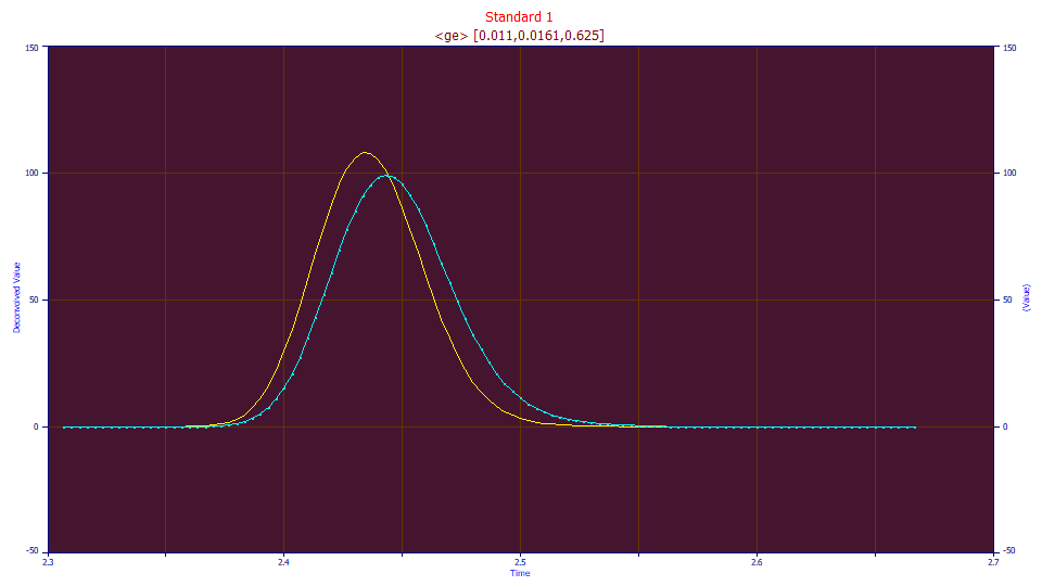
You may note the similarity to the fitted plot with the As Fitted and IRF Deconv. curves (the red and white) in the Review. A Fourier deconvolved data set will, if the noise filtering is good, allow for closed-form fits absent the IRF that will approach (but will never quite match) the fit with the IRF. In other words, the fit of the GenHVL model to the deconvolved data should be close, but not quite as good as the direct GenHVL<ge> fit. On the other hand, the closed form GenHVL fits will require virtually no fitting time, where the integral GenHVL<ge> fits will be appreciably slower.
Click OK to exit the IRF Deconvolution procedure. Click OK to accept the default titles for this new data level. There is now a second data level in the data file containing this deconvolved data. The deconvolved data set is now selected in the main window.
Fitting the IRF Removed Data
We used Fourier deconvolution to remove the IRF from the data. We can now fit the fast closed form models to this deconvolved data, and assume the instrumental/system distortions have been mathematically removed.
Fitting the GenHVL Closed Form Model
Click the Local Maxima Peaks button in the main window to open the peak placement screen.
The program remembers the prior settings. Select GenHVL as the model in the second dropdown
Click the Peak Fit button in the lower left of the dialog to open the fit strategy dialog. Select the Fit with Reduced Data Prefit, 2 Pass, Lock Shared Parameters on Pass 1. Leave the Fit using Sequential Constraints box checked. Click OK. Although we are not fitting an IRF, we are still fitting a higher order ZDD parameter. The 2-Pass option first estimates the main peak parameters while the starting estimate for the ZDD asymmetry is held constant.
Click Review Fit. You should see a fitted peak with an unaccounted variance of just 6.29 ppm, very close to the 5.17 ppm of the direct GenHVL<ge> fit. The Fourier noise filtration was effective. Click Numeric, and from the Options menu of the Numeric Summary, choose Select Only Fitted Parameters and also check Measured Values and Deconvolved Moments.
Peak�� Type�������� ������a0���� ������a1���� ������a2���� ������a3���� ������a4���� ������a5���� ������a6���� ������a7����
����1�� GenHVL<ge>�� 6.13746193�� 2.43158324�� 0.02205342�� -0.0001284�� 0.11295617�� 0.01099098�� 0.01611737�� 0.62500000
����1�� GenHVL�� ����6.13598312�� 2.43316472�� 0.02214212�� -0.0001154�� 0.10965212��
If we compare the fitted parameters, there are small differences in the higher moment a3 and a4 parameters. In the GenHVL model the a3 chromatographic distortion (the intrinsic fronting and tailing) and the a4 ZDD asymmetry both impact the skewness or third moment. If we look at the deconvolved GenHVL in the GenHVL<ge> fit and at the measured moments of the GenHVL fit of the Fourier deconvolved data, the higher order moments are close to identical.
Deconvolved�Moments
�Peak�� Type���� ���Area����� ���Mean����� ��StdDev���� �Skewness��� �Kurtosis��� �Amplitude�� ���Center�����
����1�� GenHVL�� 6.13746193�� 2.43563811�� 0.02266643�� 0.24913813�� 3.11566300�� 108.394890�� 2.43346960��
Measured�Values
�Peak�� Type���� ���Area����� ��%�Area���� ���Mean����� ��StdDev���� �Skewness��� �Kurtosis���
����1�� GenHVL�� 6.13598312�� 100.000000�� 2.43679289�� 0.02268697�� 0.24894869�� 3.11567338��
Click OK to close the Review, OK to acknowledge the name of the saved fit, OK to confirm, and OK one last time to leave the placement screen and return to main screen.
A Sampling of Gradient Peaks
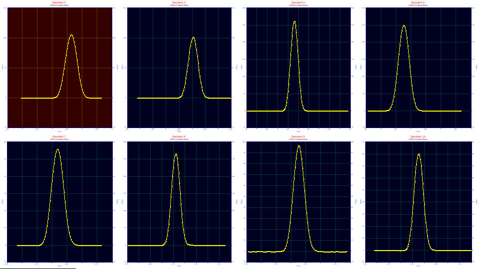
![]() Use the File menu's Open item and select the file HPLCGradientStd02.pfd from the
program's installed default data directory (\PeakLab\Data). The file contains eight data sets, each a
baseline-corrected data set from a standard which elutes during the gradient.
Use the File menu's Open item and select the file HPLCGradientStd02.pfd from the
program's installed default data directory (\PeakLab\Data). The file contains eight data sets, each a
baseline-corrected data set from a standard which elutes during the gradient.
Click on the IRF Deconvolution button and ensure the following settings are selected:
Response Fn
<e> Exponential
Deconvolve Right
IRF Parameters
0.0161
Genetic Alg Optimization
50 % (the 'e' exponential width will vary � half of its
value)
BsLnZero (we want to maximize the baseline
points)
0.50 % (the baseline region is defined as
�0.5% of the amplitude)
Fourier Filter
D2 Automatic (the FFT threshold will be determined
using a smoothed 2nd derivative)
8 (8% smoothing for the D2 algorithm)
Post-Processing
Zero Baseline Points - unchecked (baseline will be
actual subtracted values)
Zero Negative Points - unchecked (negative
baseline points are permitted)
Clearly, the 0.161 exponential tau of the isocratic IRF is far too high for the gradient peaks.
Change the value from tau value of 0.0161 to 0.01 and then to 0.008. Click the Genetic Optimize button.
![]() When the optimizations are complete, click the List Parameter Estimates button.
When the optimizations are complete, click the List Parameter Estimates button.
IRF Parm�1 ���Parm�2 ���Parm�3�������Data
<e> 0.0062723 0.0000000 0.0000000 Standard�2
<e> 0.0066746 0.0000000 0.0000000 Standard�3
<e> 0.0060608 0.0000000 0.0000000 Standard�4
<e> 0.0062490 0.0000000 0.0000000 Standard�6
<e> 0.0043381 0.0000000 0.0000000 Standard�7
<e> 0.0070402 0.0000000 0.0000000 Standard�8
<e> 0.0070539 0.0000000 0.0000000 Standard�9
<e> 0.0040000 0.0000000 0.0000000 Standard�10
Although the last data set optimized to a bound in the range set for the optimization, there is a suggestion that a measure of the exponential observed within the isocratic IRF survived the gradient compression.
Close the List window and click Cancel to exit the IRF Deconvolution procedure. We do not want to create a deconvolved data level. We merely wanted to use the genetic algorithm to estimate the measure of residual exponential distortion.
Fitting Gradient Peaks Directly to a Twice-Generalized Closed-Form Model
We will now explore the first of the three primary methods we suggest for the fitting of gradient peaks. In this tutorial, we will fit the gradient peak shape directly with closed form models where there no attempt to model or "unwind" the gradient independently, and no effort to model any residual IRF.
We will fit a twice-generalized Gen2HVL closed-form model, without an IRF, to these gradient peaks and we will achieve reasonable fits.
This simplest approach to fitting HPLC gradient peaks is discussed in the HPLC Gradient Peaks topic. In order to manage the compression of the gradient, a twice-generalized model is needed. In such models, both the third moment skew and fourth moment kurtosis in the ZDD are adjusted in the fitting. The additional fourth moment parameter very effectively estimates the gradient compression by the power of decay in the ZDD, the zero-distortion density which forms the chromatographic peaks.
By adjusting the kurtosis or fourth moment in the zero-distortion density, HPLC gradient peaks can be fitted directly with no preprocessing after baseline correction. It is a one step process from baseline-corrected data to final fitted results.
In this Gen2HVL model, the IRF, ZDD non-ideality, and the gradient will be sorted only by the third and fourth moments of the ZDD. The a3 intrinsic chromatographic distortion remains in place and is quantified to the extent it is not correlated with these lumped effects. The parameters describing the third and fourth moments will be largely orthogonal, and the gradient strength will mostly rest with the fourth moment term. The residual IRF (that which survives the gradient compression) and ZDD effects (as they exist in the presence of the gradient) will be mostly in the skew or third moment term.
As a closed form model, Gen2HVL fits are exceptionally fast as contrasted with fitting a convolution or deconvolution integral in the Fourier domain.
If needed, click the Select All button to ensure all data sets are selected. Only selected data sets are passed to the fitting procedure. Select Local Maxima Peaks from the main screen.
We will leave the settings exactly as they were set in the isocratic fit, except we will change the model to the Gen2HVL:
Peak Detection
Set Sm
n(1) to 5
Peak Type
Select Chromatography
in the first dropdown
Select Gen2HVL as the model in the second
dropdown
Scan
Set the Amp %
threshold to 1.5 %
Leave Use Baseline Segments unchecked
Be sure Use IRF,ZDD is checked
Vary
Leave width a2
and shape a3 checked, all other unchecked
We will also reset the IRF we adjusted in the isocratic fit. Click the IRF button. If you made your own modifications to the IRF defaults prior to this tutorial for your own fitting, please use the Save button to save your IRF values before resetting the defaults. Click the Defaults button. Click OK.
Click Peak Fit to open the fit strategy dialog. Select the Fit with Reduced Data Prefit, 2 Pass, Lock Shared Parameters on Pass 1. Leave the Fit using Sequential Constraints box checked. Click OK. Here the two-pass option is useful for holding the higher moment parameters constant while the main peak parameters are first estimated, and only thereafter fitting these a5 skew and a4 kurtosis-related parameters. The fits should only take no more than a second or two. Click Review Fit.
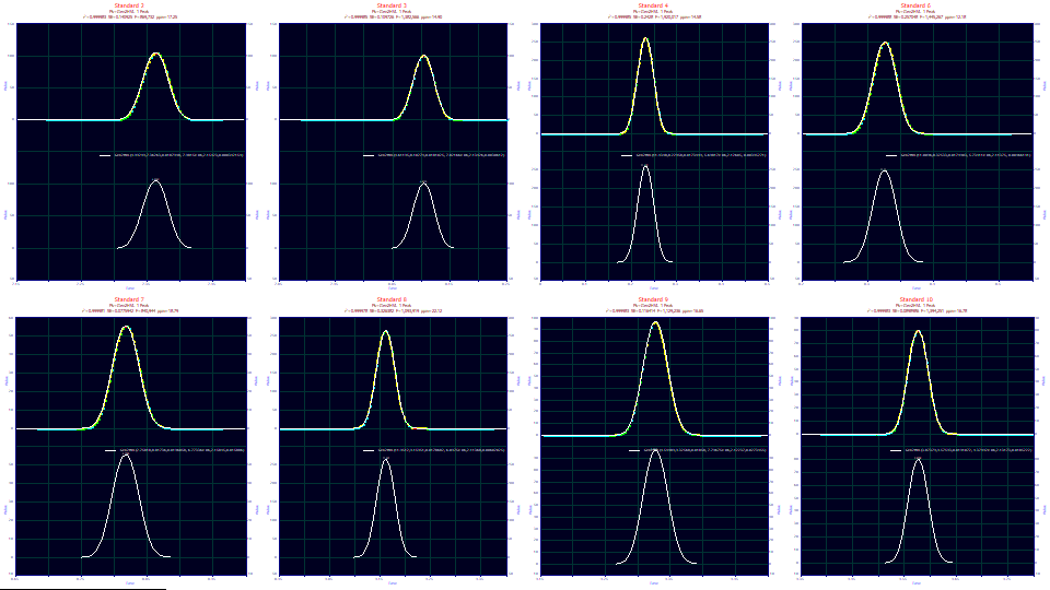
The fits vary from 12.18-22.12 ppm unaccounted variance, superb for no IRF being fitted.
If you wish to see just a single fit, double click the fit graph for the data set of interest. Double click to return to all graphs. You can also use the right click popup menu.
The gradient and remnant IRF and asymmetry will be addressed in the a5 third moment term, and the gradient power will be estimated by the a4 fourth moment kurtosis-related parameter. Click on the Numeric button to open the numeric summary. Under the Options menu, choose Select Only Fitted Parameters and then check Measured Values and Average Multiple Fits. Scroll to the end of the summary.
Average�for�8�Fits
Fitted�Parameters
r2�Coef�Det�� DF�Adj�r2���� Fit�Std�Err�� F-value������ ppm�uVar
0.99998334��� 0.99998231��� 0.17009865��� 1,259,491���� 16.6559258
�Peak�� Type����� ������a0���� ������a1���� ������a2���� ������a3���� ������a4���� ������a5����
����1�� Gen2HVL�� 6.89711574�� 8.61234579�� 0.01836171�� -6.535e-6��� 2.13181594�� 0.00782039��
Measured�Values
�Peak�� Type����� �Amplitude�� ��Center���� ���FWHM����� ��Asym50���� �FW�Base���� ��Asym10����
����1�� Gen2HVL�� 151.828576�� 8.61373910�� 0.04410695�� 0.95157334�� 0.08489044�� 0.96731930��
�Peak�� Type����� ���Area����� ��%�Area���� ���Mean����� ��StdDev���� �Skewness��� �Kurtosis���
����1�� Gen2HVL�� 6.89711574�� 100.000000�� 8.61318389�� 0.01795855�� -0.0048101�� 2.88067693��
CV�Percent�for�8�Fits
Fitted�Parameters
r2�Coef�Det�� DF�Adj�r2���� Fit�Std�Err�� F-value������ ppm�uVar
0.0002981%��� 0.0003155%��� 54.263707%��� 28.080568%��� 17.900369%
�Peak�� Type����� ������a0���� ������a1���� ������a2���� ������a3���� ������a4���� ������a5����
����1�� Gen2HVL�� 55.805236%�� 8.5877569%�� 4.3387574%�� 19.695688%�� 0.7919934%�� 147.94447%��
Measured�Values
�Peak�� Type����� �Amplitude�� ��Center���� ���FWHM����� ��Asym50���� �FW�Base���� ��Asym10����
����1�� Gen2HVL�� 59.215298%�� 8.5825204%�� 4.5662533%�� 1.9861027%�� 4.1839698%�� 2.8053694%��
�Peak�� Type����� ���Area����� ��%�Area���� ���Mean����� ��StdDev���� �Skewness��� �Kurtosis���
����1�� Gen2HVL�� 55.805236%�� 0.0000000%�� 8.5867261%�� 4.1667744%�� 656.33992%�� 0.5007086%��
The average goodness of fit is 16.6 ppm, very good for fitting no IRF. The a4 power of decay,the ZDD kurtosis-related parameter that fits the compression of the gradient within the peak, averages 2.13 with just .79 CV% (a CV coefficient of variation is the Std Deviation/Mean). An a4 of 2.0 is a Gaussian decay. The a5 asymmetry term is very low and statistically significant (different from zero) in only three of the eight fits. The a5 asymmetry modifies the zero distortion density, and here the ZDD is indeed close to symmetric. It is, however, non-Gaussian. A power of 2.13 is a strong compression (thinner, more compact tails). The orthogonal nature of the fourth moment with respect to the skew allows the strength of the gradient to be accurately mapped by this a4 parameter.
A Gaussian has a fourth moment kurtosis of 3.0. Here we average 2.88, a clear compression of the peak's tails arising from the gradient.
We note that the a2 deconvolved SD width of the peaks has a CV of just 4.3%. The standards' peaks vary little in width across time.
Especially interesting is the average and CV% of the a3 chromatographic distortion. The peaks are ever so slightly fronted, a distortion of -0.0000065, close to an infinite dilution value, but the CV is only 19.6% across the 8 samples. The samples vary from -.000004 to -.000008, all slightly fronted.
Although we fit a closed-form model (no IRF convolution integral), the gradient and a model with both higher order moments makes respectable fits possible.
Parameter a5, which addresses the skew in the zero-distortion generalized density, is widely varying across the different peaks. The statistical test of significance checks for values different from 0. When a5 fails significance, it means the fit could not distinguish the a5 as significantly different from 0. Given the symmetry in gradient peaks, this simply means that five of the above standards fit to very close to a zero ZDD asymmetry.
Click Numeric or close the Numeric Summary window directly. Click the Explore button.
![]() The Zoom-in Applies to All Graphs will probably be turned on. Click this button in the graph's
toolbar to turn this option off.
The Zoom-in Applies to All Graphs will probably be turned on. Click this button in the graph's
toolbar to turn this option off.
We'll start with the simplest relationship. Select Center (a1) for the x variable and Moments for the y variable.
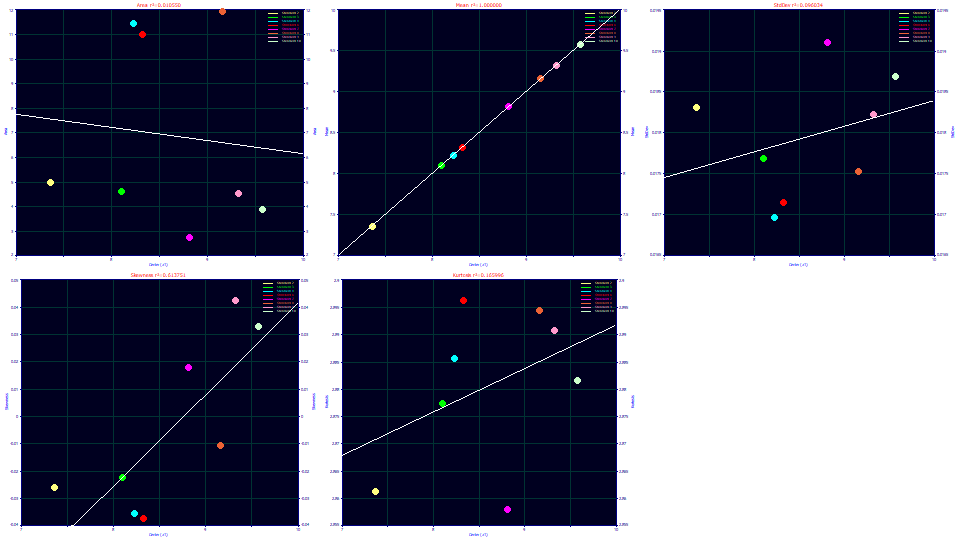
The asymmetry or skewness increases with the a1 retention time. Perhaps equally interesting is that the second moment (as a standard deviation) and the fourth moment are largely independent of retention time. In a Gen2HVL model, the a1 parameter is the first moment or mean of the generalized error zero-distortion density, the location that would be observed at infinite dilution.
Select Width (a2) for the x variable.
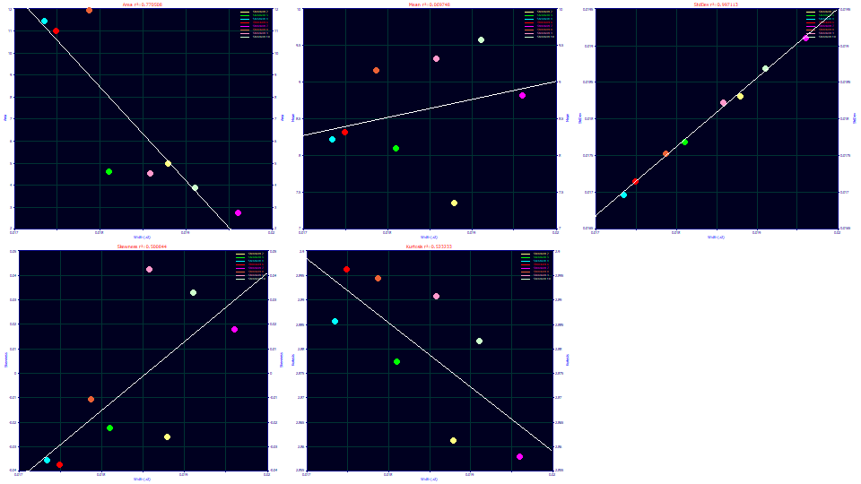
The a2 deconvolved Gaussian SD in the Gen2HVL model strongly maps to the second moment (as a SD). The relationship with skewness is generally increasing. The relationship with kurtosis is generally decreasing, and since a higher a2 width means a lower kurtosis, this means a greater width peak has thinner tails or higher compression.
Select Distortion (a3) for the x variable.
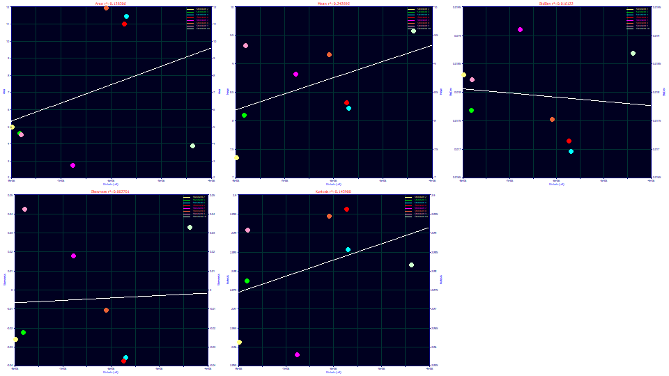
The a3 chromatographic distortion is very low in gradient fits. Here there is no clear trend with any of the overall peak moments.
Select Parameter (a4) for the x variable.
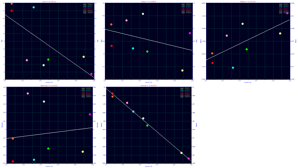
The a4 parameter in the Gen2HVL addresses the power of decay in the zero-distortion density or ZDD. It maps beautifully to the fourth moment. The orthogonality between the a4 and a5 parameters in the Gen2HVL model should have a4 independent of impact upon the skewness, and this is essentially confirmed. There is a correlation with the second moment as an SD width, but we already noted that a greater width translates to a higher fourth moment likely arising from a greater time of exposure to the gradient during its elution.
Select Parameter (a5) for the x variable. Zoom-in the gradient points to the left in each of the graphs.
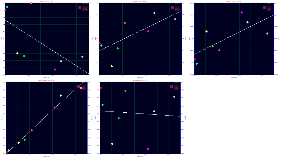
The a5 parameter in the Gen2HVL addresses the asymmetry or skew in the zero-distortion density or ZDD. It maps beautifully to the third moment. The orthogonality between the a4 and a5 parameters in the Gen2HVL model should have a5 independent of impact upon the kurtosis, and this is also confirmed. Here there is also a correlation with the second moment as an SD width, the asymmetry increasing with width, suggesting a higher third moment (right skew) may also arise from a greater time of exposure to the gradient during its elution.
Click OK to close the Explore dialog, OK to close the Review, OK to accept a saved Gen2HVL fit in the data file, OK to acknowledge the revision in the file, and OK to return to the main window.
Additional Exercises
When directly fitting the gradient peak in its compressed shape, it may not be possible to resolve the two third moment terms, the a3 describing the intrinsic chromatographic distortion, the fronting and tailing, and the a5 describing the asymmetry of the zero distortion density. Much may depend on the S/N of your data and the sampling density of the points in the data.
Fit Only One Third Moment and the Fourth Moment Parameter, the GenHVL[Q] Model
A useful exercise is to perform the above fitting with the GenHVL[Q] model (or with the Gen2HVL's asymmetry locked to 1e-12, effectively zero, in the ZDD dialog). This fits one third moment term, the a3 chromatographic distortion-there is no statistical asymmetry. If you do this you should see an average of 20.14 ppm and an F-statistic of 1.395M for these fits, in contrast with the 16.65 ppm and 1.259M of the Gen2HVL fits. The fit error is lower with the Gen2HVL but the better model by F-statistic is the one where this statistical asymmetry term is absent or zeroed. Please remember that the F-statistic is just one of many information theoretics, although it is far and away the oldest and most respected one in widespread use amongst statisticians.
Fit Only One Third Moment and the Fourth Moment Parameter, the GenError[m] Model
Another beneficial exercise is fitting the GenError[m] model. It is in both the Chromatography and Statistical families of models. The GenError[m] model also fits just one third moment term, the statistical asymmetry-there is no chromatographic distortion. You should see an average of 21.64 ppm and an F-statistic of 1.230M for these fits. The goodness of fit is poorer when only a statistical asymmetry is used to address the skewness as compared to where only the chromatographic fronting/tailing asymmetry is used, and the F-statistic is slightly weaker. This suggests the HVL and Wade-Thomas general chromatographic distortion model is more applicable to the third moment skew in gradient peaks than is the statistical asymmetry which further adjusts the chromatographic skew. We would expect the chromatographic distortion to be more prominent, and in this exercise it is, but we must point out that you are looking at effective fits and very small differences.
Fit No Higher Moment Parameters, the Gaussian Model
It is also a useful exercise to perform the above fitting using a simple Gaussian model. You can use the Normal in the Statistical family, or the Gauss model in the Chromatography family. You should see an average of 314.91 ppm unaccounted variance. You should do this just to convince yourself that the gradient peaks are not Gaussians. A gradient peak can be near-symmetric, but that does not mean the skewness and kurtosis, the higher moments necessary for a complete modeling, are those of a Gaussian. Especially with the fourth moment, it will not be so.
Fit Only the Fourth Moment, No Third Moment Parameter , the NError Model
One last exercise that may be of interest is to fit the NError model in the Statistical family. This fits a fourth moment kurtosis, but retains a zero skewness. You should see an average of 64.71 unaccounted variance for the average unaccounted variance of the eight fits.
If you take the few minutes needed to perform all of these exercises, you should readily conclude firsthand that you must account both the third and fourth moments in direct gradient peak fits. The only real question is which of the approaches you use to manage the third moment. You can fit both of the third moment parameters in the Gen2HVL, just the chromatographic distortion in the GenHVL[Q], or just the statistical asymmetry in the GenError[m] model.
In this first tutorial for gradient peak fitting, we estimated the isocratic (continuous mobile phase) <ge> IRF, the instrument/system response consisting of an area weighted half-Gaussian and first order (exponential ) as [g=0.01099, e= 0.0161, areafrac= 0.625]. We also used IRF Deconvolution to ascertain that about .006 of the .016 of the constant mobile phase exponential survived the gradient.
In the second gradient fitting tutorial, we will fit HPLC gradient peak data to a yet higher degree of modeling accuracy. Using a new fitting procedure, deconvolution fitting, we will model the gradient and deconvolve the pure chromatographic peak that would exist if no gradient existed.


 |