PeakLab v2 Documentation Contents R2N Software Home R2N Software Support
Step-by-Step 1-Variable Chromatography Expt
This will outline a basic step-by-step procedure for a 1-variable fitting experiment. In this description, we will look at an IC experiment where a Li+ peak is eluted at different concentrations. In this example, we will closely study the parametric changes with a single peak.
Step 1 - Import and Section the Data

Import the data and if necessary, section the data to include only the specific peak of interest. The actual bounds will not be critical if the baseline will be zeroed in the baseline subtraction step.
Step 2 - Baseline Correct the Data
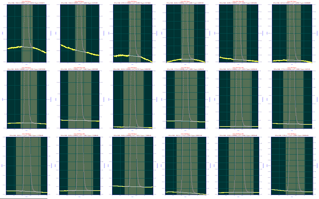
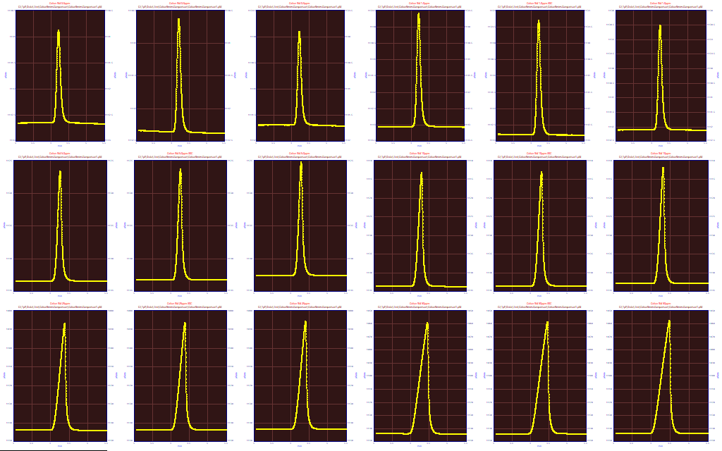
Although it requires some effort, a manual baseline specificaiton, usually with the non-parametric procedure, produces peaks that will fit to the highest possible accuracy. When there are no contaminants in the mobile phase in the region of interest, and no small coeluting components interfering with the decay on each side of the peak, the human eye will specify a baseline with an exceptional degree of accuracy.
Step 3 - View the Data to Identify any Anomalies
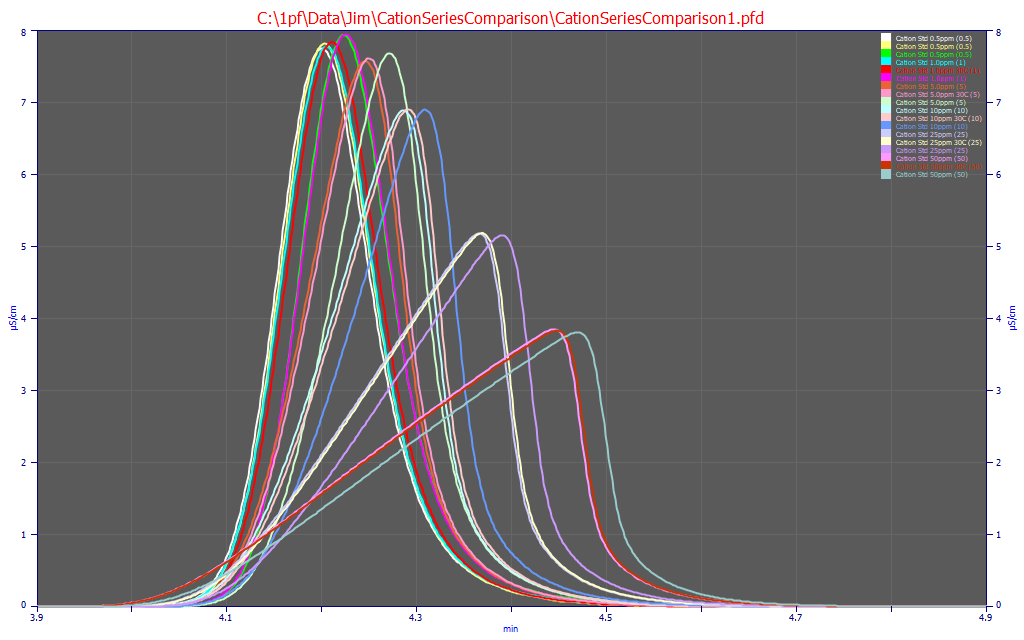
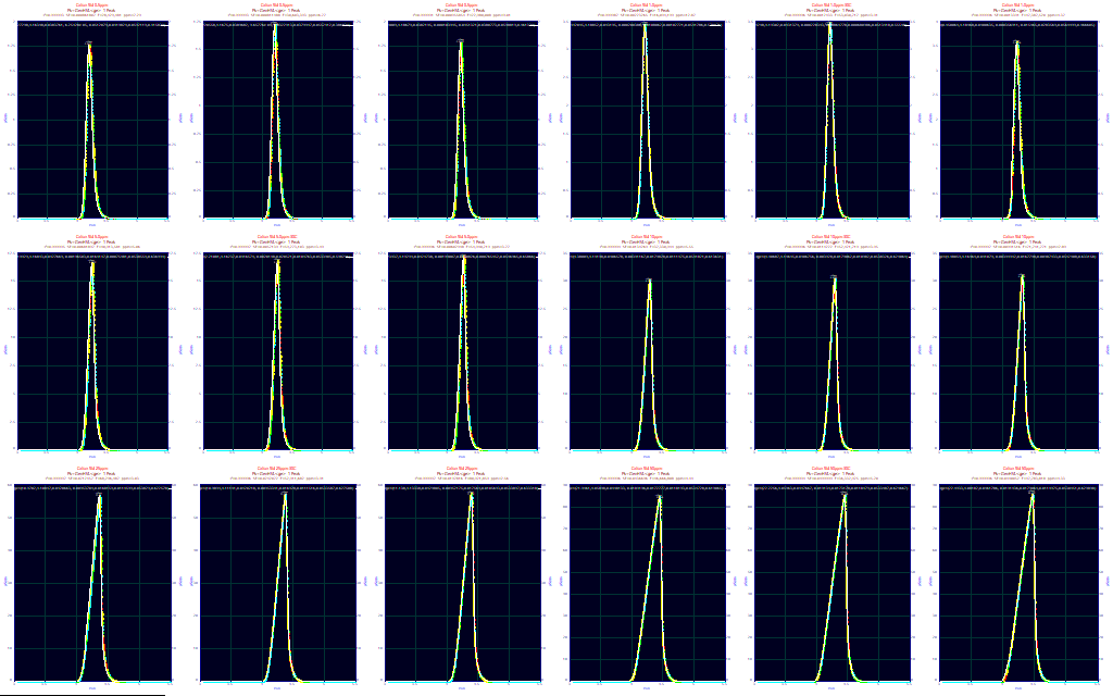
After the baselines have been corrected, you can use the View and Compare Data option to see all of the data in a single plot. Here we see two orders of magnitude in concentration from the nearly symmetric 0.5 ug/ml concentrations to sharply fronted peaks at 50 ug/ml. There are 18 chromatograms in all, three at each of the concentrations. Two of each of the three series come reasonably close to matching. One series has consistently higher elution times. This was not unexpected since these are not replicates. These three series were run at different times across more than a year. For a parametric experiment, look closely at the tailing for signs of anomalies. Those will alter the estimated parameters of the IRF (Instrument Response Function) and that will in turn alter the higher moment term(s) in the chromatographic model. Here the decay looks very clean in each of the peaks.
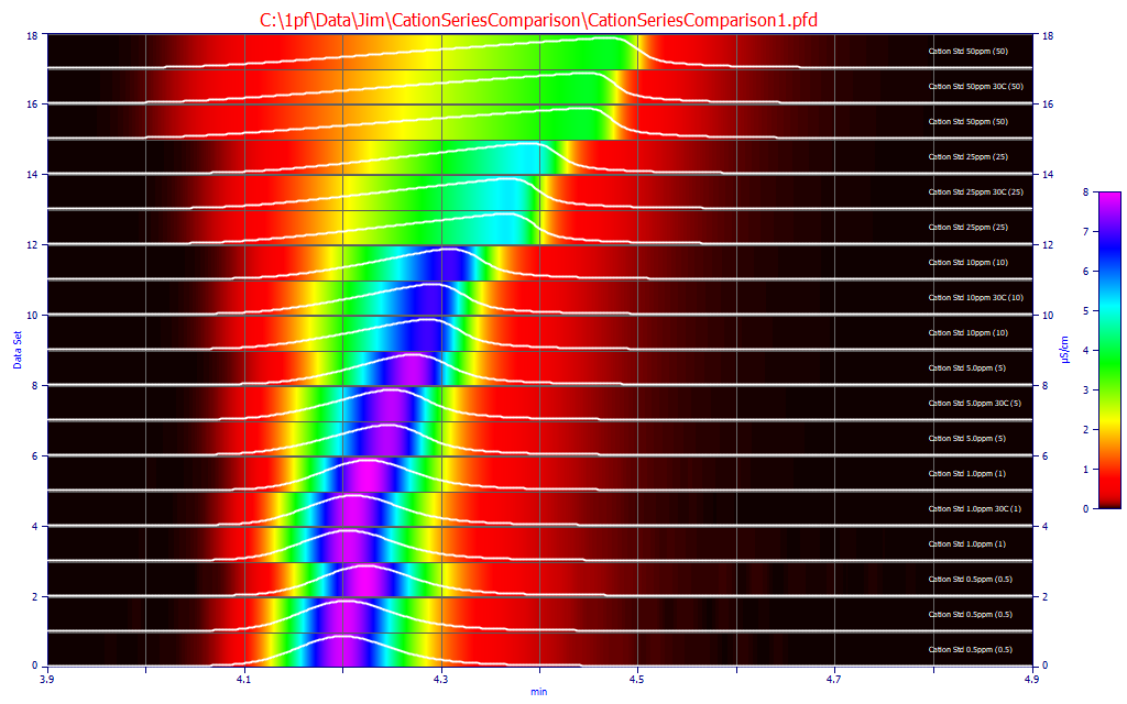
To see the subtle differences between peaks, you should use the Contour opion. The difference with the third series (the third in each sequence as you go upward in data set number) is apparent, as well as the smaller differences. Because the chromatograms are spaced across a considerable time, we will process all of these peaks in the experiment. If these were true replicates, a much more rigorous consistency might well be imposed.
Step 4 - Fit the Data to a Once Generaralized Chromatographic Model
If you wish to see statistical widths and asymmetries, as is most often the case, we recommend you start with the GenHVL model.
In this IC data where the peaks can be modeled with first order kinetics, we recommend the GenNLC model.
The GenHVL and GenNLC models will each fit a given peak to an identical goodness of fit. For the GenHVL, the a2 width is a Gaussian SD, and the a4 third moment term is a standard statistical asymmetry that varies from -1 to 1. For the GenNLC, the a2 is a first order kinetic time constant, and the a4 asymmetry is indexed to the NLC's asymmetry where an a4=1/2 exactly reproduces the NLC. For the GenHVL and GenNLC, the a3 chromatographic distortion, the concentration-dependent tailing or fronting, is identical for the two models.
We also recommend that you start with the <ge> IRF. This contains a half-Gaussian probabilitistic component to model the axial dispersion and a first order exponential to model in the aggregate all kinetic delays in the system. For short length columns, there may be two kinetic components that dominate the iinstrumental ninidealities, and in this case you may wish to also include the <e2> IRF.
Step 5 - Assess the Goodness of Fit
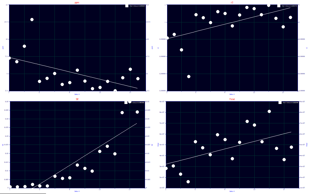
We recommend that you liberally use the Explore feature to graphically evaluate your chromatographic experiments. This is the Fit Statistics vs Data # set of plots. The first panel shows the ppm statistical (least-squares) error. This is simply 1e6*(1-r2). In this example the errors are higher at the lower concentrations, as might be expected, but the worst error is about 12.9 ppm and the best is 2.9 ppm. The worst r2 is 0.999987. You should be especially wary of parametric comparsions where an inferred trend occurs across wide variations in goodness of fit.
Step 6 - View the Parametric Comparisons
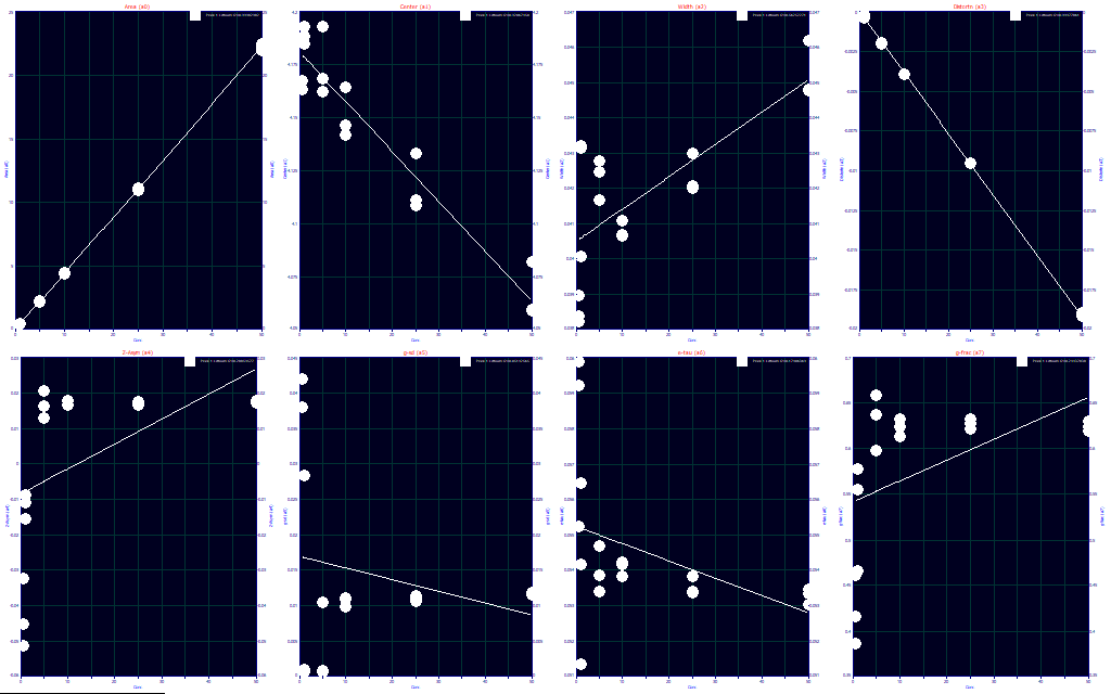
In order for PeakLab to know the specific values of the experimental variables, you must right click in the main window or in the Review and select the Map Experimental Process Variables for Fitted Data Sets option. Once these variables have been entered, they will be available to the Explore option. Here we have concentration on the X-axis, and the a0 - a7 parameters in the Y-axis of the eight plots. This is where an experiment is graphcally evaluated with respect to the fit parameters.
For example, the first plot of a0 illustrates that the area is linearly proportional to concentration, as expected.
The second plot is of a1, the center parameter, and it shows a small but consistent trend of earlier elution with concentration. The a1 is the center of mass of the infinite dilution peak with all instrumental distortions removed, but with this a4 third moment core density asymmetry accounted. Because this center will be independent of the IRF, which may vary with experimental variables, and it is also independent of the chromatographic tailing/fronting arising from concentration differences, you can see a1 as a true center of the elution for the separation.
The third plot is of a2, the width parameter. For this GenHVL model, we have a Gassian SD. This is the width of the generalized normal upon which the model is formed. This width is independent of the IRF, the chrmatographic tailing and fronting, and the asymmetry. It can be seen as a true measure of the amount of broadening in the separation.
The fourth plot contains the the a3 estimate of chromatographic tailing and fronting arising from the concentration dependence on peak shape. In a generalized chromatographic model, there are two terms that deal with the shape of the peak. In the GenHVL, the a3 models the HVL and NLC tailing and fronting, and a4 the third moment statistical deviation from a Gaussian. In this IC concentration series, the Haarhoff-VanderLine and Wade-Thomas theoretical parametric estimate of tailing and fronting is almost perfectly linear with concentration, a complete validation of HVL and NLC theory. Because this peak is intrinsically fronted (a3 is negative), it becomes more fronted, more negative, with concentration. If this peak were intrinsically tailed (a3 positive), it would become more tailed, a higher positive a3 parameter value, with concentration.
The fifth plot contains the a4 estimate of infinite dilution density asymmetry. In HPLC, this is strongly impacted by the packing of the media in the column as well as the uniformity of pore size in the media. Here in this IC study, we see essentially a constant value of 0.015, a very small right asymmetry, at all concentrations ranging from 5 to 50 ug/ml. The 0.5 and 1 ug/ml concentrations in this study do not track and may be related to the much lower S/N in the data.
The sixth, seventh, and eight plots contain the IRF estimates. Here we see a very high variability on the low S/N samples, but near constant results for the higher 5-50 ug/ml concentrations. The probabilisitic component, a5, the kinetic component, a6, and the area fraction of the probabilisitic component, a7 are nearly constant. When the S/N was high enough to be deemed reliable, the a4 infinite dilution asymmetry, and the IRF parameters, appear to be independent of concentration.