PeakLab v1 Documentation Contents AIST Software Home AIST Software Support
Two-State Experimental Models (Tutorial)
Closed-Form Models that Fully Manage the Real-World Chromatographic Shape
Much of the UDF capability in PeakLab was born of our wanting to find a way to fit the eluted shape of a chromatographic peak to close to zero error using a complete closed form solution. We will share at the outset we were never successful with isocratic peaks to the extent of the IRF fits, such as the Generalized HVL and Generalized NLC models with the <ge> and <e2> IRFs which manage analytic peaks with close to zero error.
We will assert that we believe the true shape of most chromatographic peaks to be a convolution integral of a two-component system IRF and a peak consisting of the common chromatographic operator applied to a zero-distortion density, usually one with at least a third moment skewness generalization.
If we step away from that convolution integral, it means the entirety of that two-component IRF must be modeled by complex changes to the ZDD zero distortion density. To accomplish this, we must create at least a two-state ZDD. In creating these two state models, our original intention was to have one state manage the core peak shape and the other state strictly manage the IRF tailing. The premise was straightforward. We know the peak minus the IRF is beautifully described by the chromatographic distortion operator applied to a generalized normal default or [Z] ZDD. We only needed to seed in a second ZDD component whose sole function would be to produce as much of this IRF tailing as possible.
As you will note in this tutorial, perhaps with some humor, an interesting aspect of non-linear fitting is that the minimization hardly respects expectations.
In PeakLab, two component ZDD models are designated similar to the following: GenHVL2[Z|E]. That which we see as the principal or primary component is managed by the [Z] density, and the secondary component is managed by the [E] density. For this approach to work, we must be able to specify the relative amounts of the two components. We chose to construct the built-in two state models by specifying the fraction of the secondary component, the one we intended to specifically seed into the overall ZDD to reproduce the IRF tailing.
Note the subtle differences in the PeakLab model nomenclature. A Gen2HVL model is twice generalized, often a fourth moment adjustment added to the third moment adjustment in a single ZDD. A GenHVL2 model uses a two-component ZDD where the two different ZDD components are separated by the | symbol.
The GenHVL2[Z|E] and GenHVL2[Z|G] Models
The GenHVL[Z] is a variation of the GenHVL where the a1 is the mean of the deconvolved Gaussian or normal upon which the generalized normal is structured. The difference between the GenHVL and the GenHVL[Z] is only in the a1 center parameter and it is usually negligible since small changes in the ZDD produce large differences in the overall chromatographic shape. Still, to have both states in a two-state model wholly coherent, we chose to have the a1 be the deconvolved Gaussian mean, and a2 to be the deconvolved Gaussian SD, for both states in all of the built-in two state models. All of the two-state models will thus use the [Z], [Y], or [Q] ZDD as the main peak component. These reduce to a Gaussian where the a1 is the mean and a2 is the SD of that Gaussian, the [Z] doing so with zero asymmetry, the [Q] doing so with a power of 2 Gaussian decay, and the [Y] doing so with both of these specializations.
In both the GenHVL2[Z|E] and GenHVL2[Z|G] models, the two densities share a common a1 center and a2 width and there are two additional parameters as compared to the GenHVL, this exponential time constant or SD width of the EMG or GMG, and a fraction of this second component specified as the base 10 log of the fraction. A fraction specified as -2 would mean the second component EMG or GMG would be present in the ZDD at a 0.01 fraction of the overall area of the ZDD.
The GenHVL[Z|E] experimental model is thus a synched a1 and a2 blend of the [Z] ZDD and [E] ZDD. The GenHVL[Z|G] is a synched a1 and a2 blend of the [Z] ZDD and [G] ZDD. Note that there is a shift in the parameter sequence in these models. The a4 becomes the base 10 log fraction of the second component. The other primary ZDD parameters then follow, and finally the secondary ZDD parameters. For the [Z|E] and [Z|G] models, the a5 parameter becomes the principal statistical asymmetry in the [Z] component of the density and the a6 parameter will either be the exponential time constant of the EMG or half-Gaussian SD of the GMG.
Sample Data for the Two-State Fit
![]() From the File menu, select Open... (or use the main toolbar Open button) and the
choose the file TwoStateTutorial.pfd from the program's installed default data directory (\PeakLab\Data).
From the File menu, select Open... (or use the main toolbar Open button) and the
choose the file TwoStateTutorial.pfd from the program's installed default data directory (\PeakLab\Data).
Right click the main graph and select the Replicate this Data Set a Specified Number of Times from the popup menu. Enter 5 for the count of replicates and click OK. You should now have four identical data sets in the main window.
![]() Click the Local
Maxima Peaks button in the main window (or you can use the Fit Local Maxima Peaks... in
the Peaks menu or main toolbar).
Click the Local
Maxima Peaks button in the main window (or you can use the Fit Local Maxima Peaks... in
the Peaks menu or main toolbar).
Set the placement options as follows. Most are the defaults:
Peak Type
Set
Sm n(1) to 20 (the
one-sided smoothing window)
Peak Type
Select Chromatography
All in the first dropdown
Select GenHVL as the model in the second dropdown
Scan
Set the Amp %
threshold to 1.5 %
Leave Use Baseline Segments unchecked
Be sure Use IRF,ZDD is checked
Vary
Leave width a2
and shape a3 checked. Leave
all others unchecked.
Click the IRF button. If you made modifications to the IRF defaults prior to this tutorial for your own fitting, please use the Save button to save your IRF values before resetting the defaults. Click the Defaults button. Click OK.
Click the Model Experiment button. In a model experiment, multiple models are fit to identical replicates of data allowing you to rapidly compare the different models in a single Review.
Select the following models from the list:
HVL
GenHVL
HVL<ge>
GenHVL<ge>
GenHVL<e>
GenHVL2[Z|E] (about a third of way down the list)
The dialog will show Models (6 selected). Click OK. There are now four different
placements based on the four models in the model experiment.
The first fit will be the HVL model. This is our reference for the theoretical peak being fitted absent the IRF and all higher moment ZDD adjustments. This is a closed-form fit.
The second fit will be the GenHVL model. This is our reference for the generalized peak being fitted absent the IRF but with the third moment skewness adjustments in the ZDD. This is a closed-form fit.
The third fit will be the HVL<ge> model. This is our reference for the theoretical peak with no ZDD adjustments but with a two-component IRF fully fitted. This is a convolution integral fit in the Fourier domain.
The fourth fit will be the GenHVL<ge> model. This is our target reference for the generalized peak with the third moment ZDD and two-component IRF fully fitted. This is a convolution integral fit in the Fourier domain.
The fifth fit will be the GenHVL<e> model. This is our reference for the generalized peak with the third moment ZDD and an IRF fitted with only a single component exponential. This is also a convolution integral fit in the Fourier domain.
The sixth fit will be the GenHVL2[Z|E] two-state model where the second component of the density is the EMG. No IRF is fitted. This is a closed-form fit.
Right click the sixth graph and select the Set Common Parameters Across Peaks for this Data Set... item in the popup.
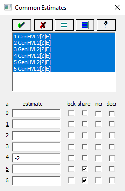
![]() Click the Select All Peaks button. Enter -2 for the a4 parameter and uncheck
the share (if needed). We are setting a starting estimate for a4 where 10^-2 or 0.01
of the overall density consists of the second component, the EMG, and 0.99 consists of the primary component,
the generalized normal. Unfortunately, for two-state models, it will be necessary for a4, this
area fraction of the second component, to vary for each peak in the data set.
Click the Select All Peaks button. Enter -2 for the a4 parameter and uncheck
the share (if needed). We are setting a starting estimate for a4 where 10^-2 or 0.01
of the overall density consists of the second component, the EMG, and 0.99 consists of the primary component,
the generalized normal. Unfortunately, for two-state models, it will be necessary for a4, this
area fraction of the second component, to vary for each peak in the data set.
![]() Click the OK button to accept the changes.
Click the OK button to accept the changes.
Click the Peak Fit button in the lower left of the dialog to open the fit strategy dialog. Select the Fit with Reduced Data Prefit, Cycle Peaks, 2 Pass, Lock Shared Parameters on Pass 1. Be sure the Fit using Sequential Constraints box checked. Click OK.
You will may note that the GenHVL in the first data set finishes first, then the two state models, and finally the IRF convolution integral models.
Click Review Fit.
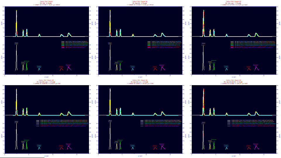
There are immense differences in unaccounted variance:
HVL (no ZDD, no IRF) 3929 ppm
GenHVL (ZDD, no IRF) 3915 ppm
HVL<ge> (no ZDD, two-component IRF) 52.6 ppm
GenHVL<ge> (ZDD, two-component IRF) 8.06 ppm
GenHVL<e> (ZDD, one-component IRF) 738 ppm
GenHVL2[Z|E] (2-component ZDD, no IRF) 46.8 ppm
This model experiment highlights the different model paradigms, placing each in perspective. In this experiment, our target for the two-state models is to reproduce the fit of the GenHVL<ge> model with its full third-moment adjustment in the ZDD, and its very capable two-component <ge> IRF. As the results indicate, the inclusion of the second ZDD component, the [E], is impressive even if it cannot match the target. Of all the closed form models explored during PeakLab's development, none came close to these two-state ZDD models. Given that the 3929 ppm in the HVL in the first data set represents the best achievable fit with the earlier versions of the product, there was a point prior to the refinements in the IRF modeling, where we would have been overjoyed with that 47 ppm in the two-state fit. It is no small achievement to outperform the HVL<ge> convolution model with a closed form model.
We should note that the two-state models are not of the same fitted parameter count as the convolution models which add just three (<ge>) parameters to the four HVL parameters for each of the six peaks. In a two-state model, the second component fraction must vary with the peaks in the elution. The GenHVL<ge> adds four parameters to the 24 HVL parameters, for a total of 28. The GenHVL2[Z|E] fit adds 8 parameters, for a total of 32.
This is another example that illustrates how important a two-component IRF and third-moment ZDD adjustment are in modeling analytic peaks.
Double click the fourth graph.
![]() Click the Hide Y plot in the graph's toolbar. Use the mouse to zoom in just the first peak.
Look closely, you will have to zoom in multiple times to see differences between the model and data. This
is what a 8 ppm fit looks like. Right click and select Restore Scaling - Undo Zoom. Zoom-in
as many peaks as you like.
Click the Hide Y plot in the graph's toolbar. Use the mouse to zoom in just the first peak.
Look closely, you will have to zoom in multiple times to see differences between the model and data. This
is what a 8 ppm fit looks like. Right click and select Restore Scaling - Undo Zoom. Zoom-in
as many peaks as you like.
Double click the graph to restore all plots.
Double click the sixth graph.
![]() Click the Hide Y plot in the graph's toolbar. Use the mouse to zoom in just the first peak.
You will see small differences near the apex and in the tailing. This is what a 47 ppm fit
looks like. Right click and select Restore Scaling - Undo Zoom.
Click the Hide Y plot in the graph's toolbar. Use the mouse to zoom in just the first peak.
You will see small differences near the apex and in the tailing. This is what a 47 ppm fit
looks like. Right click and select Restore Scaling - Undo Zoom.
Double click the graph to restore all plots.
In the second dropdown, select State-1. In the third dropdown, select State-2. Double click the sixth graph.
![]() Click the Hide Y2 plot in the graph's toolbar. Use the mouse to zoom in just the peak.
Click the Hide Y2 plot in the graph's toolbar. Use the mouse to zoom in just the peak.

Click Numeric to open the Numeric Summary, Choose Select Only Fitted Parameters from the Options menu, and also select the Advanced Area Analysis option.
Fitted�Parameters
r2�Coef�Det�� DF�Adj�r2���� Fit�Std�Err�� F-value������ ppm�uVar
0.99995317��� 0.99995303��� 0.01658610��� 7,645,157���� 46.8332718
�Peak�� Type���������� ������a0���� ������a1���� ������a2���� ������a3��� ������a4���� ������a5���� ������a6����
����1�� GenHVL2[Z|E]�� 3.57993894�� 2.34126794�� 0.03410183�� -0.0052181�� -2.7827701�� -0.0061587�� 0.03383155��
����2�� GenHVL2[Z|E]�� 1.00074630�� 3.77585034�� 0.03988940�� -0.0010597�� -0.4530348�� -0.0061587�� 0.03383155��
����3�� GenHVL2[Z|E]�� 1.15868258�� 4.54754968�� 0.04539491�� -0.0003816�� -0.1801598�� -0.0061587�� 0.03383155��
����4�� GenHVL2[Z|E]�� 0.52659443�� 7.22144357�� 0.07476425�� 0.00092784�� -0.0834855�� -0.0061587�� 0.03383155��
����5�� GenHVL2[Z|E]�� 0.89013459�� 11.9756850�� 0.13812015�� 0.00578829�� -0.0002017�� -0.0061587�� 0.03383155��
����6�� GenHVL2[Z|E]�� 1.82386774�� 13.6587337�� 0.15382917�� 0.01200940�� -4.343e-7��� -0.0061587�� 0.03383155��
Advanced�Area�Analysis
�Peak�� Type���������� ����Area���� ��%�Area���� �ApexAsym��� �Area�State1 ���%�Area��� �Area�State2 ���%�Area���
����1�� GenHVL2[Z|E]�� 3.57993894�� 39.8658470�� 0.53637592�� 3.13649970�� 87.6132178�� 0.44343924�� 12.3867822��
����2�� GenHVL2[Z|E]�� 1.00074630�� 11.1442121�� 0.98701190�� 0.51050321�� 51.0122507�� 0.49024309�� 48.9877493��
����3�� GenHVL2[Z|E]�� 1.15868258�� 12.9029749�� 1.06217352�� 0.35412290�� 30.5625465�� 0.80455967�� 69.4374535��
����4�� GenHVL2[Z|E]�� 0.52659443�� 5.86410362�� 1.22115436�� 0.10259739�� 19.4831887�� 0.42399704�� 80.5168113��
����5�� GenHVL2[Z|E]�� 0.89013459�� 9.91245102�� 1.61205248�� 0.00051222�� 0.05754356�� 0.88962237�� 99.9424564��
����6�� GenHVL2[Z|E]�� 1.82386774�� 20.3104113�� 2.25687444�� 2.5529e-6��� 0.00013997�� 1.82386519�� 99.9998600��
��All�� Total��������� ������������ ������������ ������������ 4.10423796�� 45.7043893�� 4.87572660�� 54.2956107��
This is where it gets quite interesting. We wanted the Z component of the ZDD to model just the pure chromatographic peak, and the E component only the IRF, and we were even hoping to see close to the same time constant for the exponential in the EMG as in the reference fit's IRF in the second data set. We actually come somewhat close in this GenHVL2[Z|E] fit, a value of 0.034 for the EMG's width as compared to 0.043 exponential in the GenHVL<ge> IRF. We did not expect to see the immense differences in partitioning, peak to peak.
In peak 1, the [Z] state 1 component, the red GenHVL[Z] peak, is 88% of the overall area. The [E] state two component, the green GenHVL[E] peak, is 12% of the overall peak area. In peak 2, the areas are close to equal, and in peak three the green peak now predominates with 70% of the area, despite the peak being slightly intrinsically fronted (a3<0). By peak four, the GenHVL[E] is 80% of the ZDD area. For the highly tailed peaks 5 and 6 the GenHVL[E] has almost wholly overtaken the peak (the red GenHVL[Z] peak is too small to plot, and the green GenHVL[E] peak is overlaid by the overall peak.
This is the main point we want to make with respect to two state models. There is a partitioning that will occur across the two densities. If allowed to freely move about in parameter space, this two-state model changes in partition from nearly a GenHVL[Z] to a GenHVL[E] across the eluted peaks.
A constant blend in the ZDD can be enforced by sharing a4 across peaks.
Double click the graph to restore all plots. Click OK. Click OK to accept the default name and OK again to acknowledge the revision to the data file. You will be back in the placement screen.
Right click the sixth graph and again select the Set Common Parameters Across Peaks for this Data Set... item in the popup.
![]() Click the Select All Peaks button. Enter -2 for the a4 parameter and check
the share. Click the OK button to accept the changes.
Click the Select All Peaks button. Enter -2 for the a4 parameter and check
the share. Click the OK button to accept the changes.
Right click the sixth graph and select the Fit this Data Set... item in the popup.
Select the Fit with Reduced Data Prefit, Cycle Peaks, 2 Pass, Lock Shared Parameters on Pass 1. Be sure the Fit using Sequential Constraints box checked. Click OK.
As a closed form model, the fit should be quite fast. Click Review Fit. Click OK to acknowledge that the Review will reflect a differing state of fits. Only the last fit will be changed.
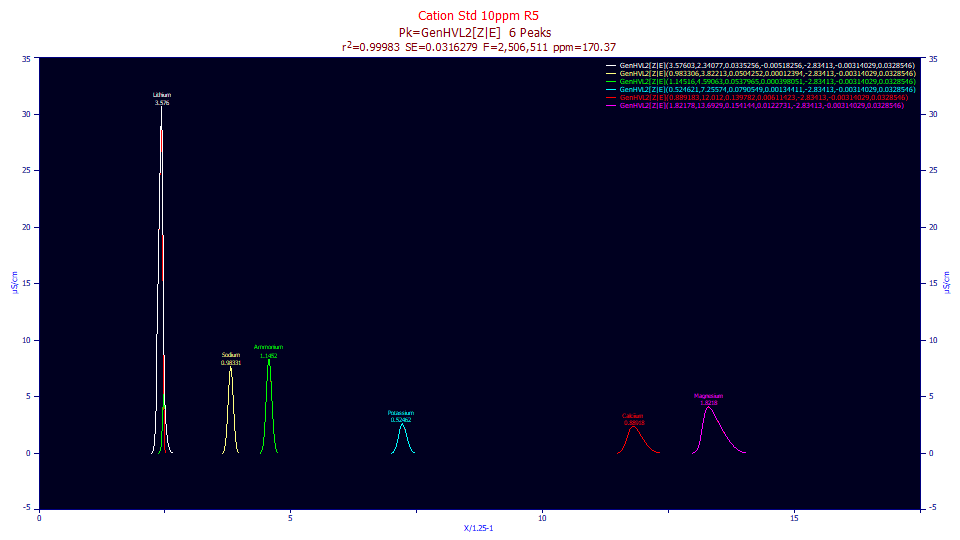
The goodness of fit diminished from 47 ppm error to 170 ppm. Here we see the two components visually on only the first peak. Peaks 2-6 are almost completely GenHVL[Z] peaks.
Zoom in the baseline.
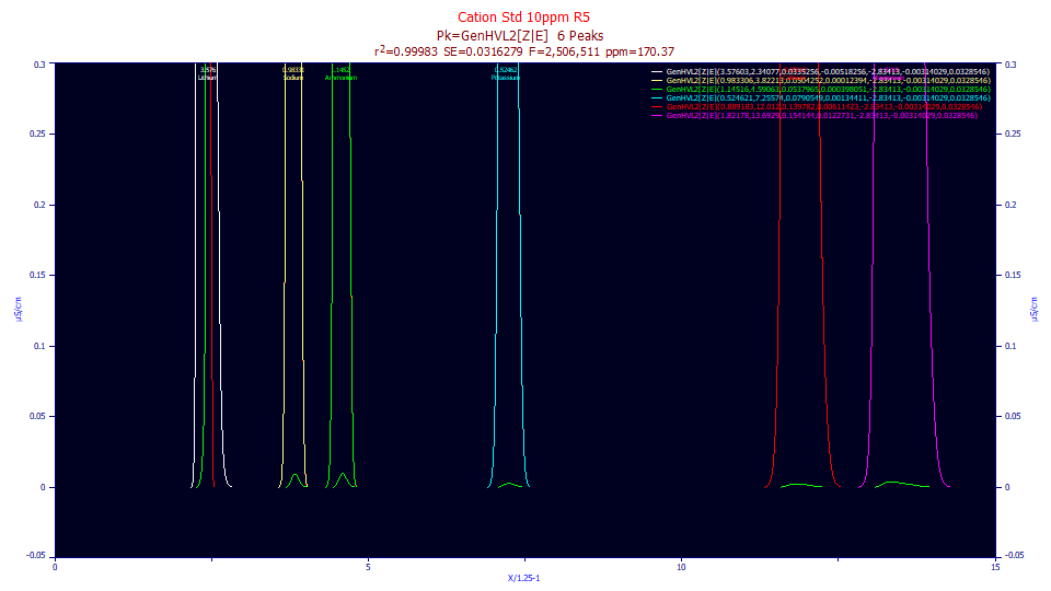
Here we see the GenHVL[E] components in the green baseline peaks.
Click Numeric to open the Numeric Summary, choose Select Only Fitted Parameters from the Options menu, and also select the Advanced Area Analysis option.
Fitted�Parameters
r2�Coef�Det�� DF�Adj�r2���� Fit�Std�Err�� F-value������ ppm�uVar
0.99982963��� 0.99982921��� 0.03162787��� 2,506,511���� 170.373318
�Peak�� Type���������� ������a0���� ������a1���� ������a2���� ������a3��� ������a4���� ������a5���� ������a6����
����1�� GenHVL2[Z|E]�� 3.57603493�� 2.34076846�� 0.03352558�� -0.0051826�� -2.8341299�� -0.0031403�� 0.03285462��
����2�� GenHVL2[Z|E]�� 0.98330601�� 3.82212607�� 0.05042518�� 0.00012394�� -2.8341299�� -0.0031403�� 0.03285462��
����3�� GenHVL2[Z|E]�� 1.14516221�� 4.59062826�� 0.05379652�� 0.00039805�� -2.8341299�� -0.0031403�� 0.03285462��
����4�� GenHVL2[Z|E]�� 0.52462101�� 7.25573738�� 0.07905493�� 0.00134411�� -2.8341299�� -0.0031403�� 0.03285462��
����5�� GenHVL2[Z|E]�� 0.88918253�� 12.0119724�� 0.13978233�� 0.00611423�� -2.8341299�� -0.0031403�� 0.03285462��
����6�� GenHVL2[Z|E]�� 1.82178489�� 13.6928702�� 0.15414412�� 0.01227312�� -2.8341299�� -0.0031403�� 0.03285462��
Advanced�Area�Analysis
�Peak�� Type���������� ����Area���� ��%�Area���� �ApexAsym��� �Area�State1 ���%�Area��� �Area�State2 ���%�Area���
����1�� GenHVL2[Z|E]�� 3.57603493�� 39.9999810�� 0.53329864�� 3.13244484�� 87.5954764�� 0.44359010�� 12.4045236��
����2�� GenHVL2[Z|E]�� 0.98330601�� 10.9988360�� 1.02102778�� 0.98190654�� 99.8576772�� 0.00139947�� 0.14232285��
����3�� GenHVL2[Z|E]�� 1.14516221�� 12.8092895�� 1.08477502�� 1.14362935�� 99.8661450�� 0.00153286�� 0.13385503��
����4�� GenHVL2[Z|E]�� 0.52462101�� 5.86818386�� 1.22872101�� 0.52396219�� 99.8744194�� 0.00065882�� 0.12558062��
����5�� GenHVL2[Z|E]�� 0.88918253�� 9.94601138�� 1.61610786�� 0.88812100�� 99.8806179�� 0.00106152�� 0.11938211��
����6�� GenHVL2[Z|E]�� 1.82178489�� 20.3776983�� 2.26441046�� 1.81982276�� 99.8922959�� 0.00196214�� 0.10770406��
��All�� Total��������� ������������ ������������ ������������ 8.48988668�� 94.9642025�� 0.45020491�� 5.03579749��
The area of the second component is 12% on the first peak, as prior, but the second component area of peaks 2-6 are all about .1%. A ZDD's components will not enter evenly into the a3 distortion transform which produces the chromatographic shape.
When fitting a two-component model a given component can have close to no effect, if it is effectively buried in the other density. The effect can be pronounced if the component has a presence where the other is very small or essentially zero. To use these experimental models, as they presently exist, a4 will have to be varied across the peaks. Note that the first three peaks, which we know are intrinsically fronted, fit here with only the first of these peaks fronted and the second and third tailed.
We will make one more fit with these experimental models.
Click OK to restore all plots, OK to exit the Review, OK to accept the default name for the fit, and OK to acknowledge the change to the data file, and OK once more to return to the main screen.
The GenHVL2[Z|GE] Model
The GenHVL2[Z|GE] model offers a second state component that is an area sum of the EMG and GMG which should at least in principle be closer to the <ge> IRF.
Click Unselect All. We only want to fit this one model. Only selected data sets are passed to the fitting procedure.
![]() Click the Local
Maxima Peaks button in the main window (or you can use the Fit Local Maxima Peaks... in
the Peaks menu or main toolbar).
Click the Local
Maxima Peaks button in the main window (or you can use the Fit Local Maxima Peaks... in
the Peaks menu or main toolbar).
From the Chromatography All family select the GenHVL2[Z|GE] model. In the Vary section check a4. Be sure the Use IRF,ZDD Config item is checked.
Right click the graph and select the Set Common Parameters Across Peaks for this Data Set... item in the popup.
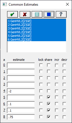
![]() Click the Select All Peaks button. Enter -2 for the a4 parameter and uncheck
the share (if needed). Enter .1 for a6, .1 for a7, and .75 for
a8. These aren't particularly close, but when working with IRF type parameters, it is sometimes
necessary to overspecify lengths. If these are too small and have too little an impact on a model, it
may take many iterations to get to the minimum.
Click the Select All Peaks button. Enter -2 for the a4 parameter and uncheck
the share (if needed). Enter .1 for a6, .1 for a7, and .75 for
a8. These aren't particularly close, but when working with IRF type parameters, it is sometimes
necessary to overspecify lengths. If these are too small and have too little an impact on a model, it
may take many iterations to get to the minimum.
![]() Click the OK button to accept the changes.
Click the OK button to accept the changes.
Click the Peak Fit button in the lower left of the dialog to open the fit strategy dialog. Select the Fit with Reduced Data Prefit, Cycle Peaks, 2 Pass, Lock Shared Parameters on Pass 1. Be sure the Fit using Sequential Constraints box checked. Click OK.
You will may note that the GenHVL in the first data set finishes first, then the two state models, and finally the IRF convolution integral models.
Click Review Fit when the fit is finished.
![]() Click the Hide Y2 plot in the graph's toolbar. Use the mouse to zoom in just the peak.
Click the Hide Y2 plot in the graph's toolbar. Use the mouse to zoom in just the peak.
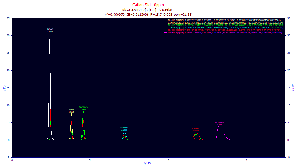
The fit has a 21.3 ppm error and the F-statistic is about twice that of the GenHVL2[Z|E] model. Further the red GenHVL[Z] is present in five of the six peaks. The green GenHVL[E] increases with each peak and it is again essentially complete for the last of the six peaks.
If needed, click Numeric to open the Numeric Summary, choose Select Only Fitted Parameters from the Options menu, and also select the Advanced Area Analysis option.
Fitted�Parameters
r2�Coef�Det�� DF�Adj�r2���� Fit�Std�Err�� F-value������ ppm�uVar
0.99997865��� 0.99997858��� 0.01120057��� 15,749,025��� 21.3534383
�Peak�� Type����������� ������a0���� ������a1���� ������a2���� ������a3���� ������a4���� ������a5���� ������a6���� ������a7� ������a8����
����1�� GenHVL2[Z|GE]�� 3.59027436�� 2.33977858�� 0.03335613�� -0.0052983�� -3.1372734�� -0.0050143�� 0.05437925�� 0.05450196 0.82258356��
����2�� GenHVL2[Z|GE]�� 1.00013406�� 3.78172979�� 0.04149280�� -0.0009886�� -0.6585085�� -0.0050143�� 0.05437925�� 0.05450196 0.82258356��
����3�� GenHVL2[Z|GE]�� 1.15977610�� 4.55495936�� 0.04663129�� -0.0003972�� -0.4762694�� -0.0050143�� 0.05437925�� 0.05450196 0.82258356��
����4�� GenHVL2[Z|GE]�� 0.52686177�� 7.22409200�� 0.07414454�� 0.00086304�� -0.2750552�� -0.0050143�� 0.05437925�� 0.05450196 0.82258356��
����5�� GenHVL2[Z|GE]�� 0.89019510�� 11.9737766�� 0.13694927�� 0.00571287�� -0.0972602�� -0.0050143�� 0.05437925�� 0.05450196 0.82258356��
����6�� GenHVL2[Z|GE]�� 1.82401272�� 13.6473428�� 0.15314915�� 0.01190615�� -4.343e-7��� -0.0050143�� 0.05437925�� 0.05450196 0.82258356��
Advanced�Area�Analysis
�Peak�� Type����������� ����Area���� ��%�Area���� �ApexAsym��� �Area�State1 ���%�Area��� �Area�State2 ���%�Area���
����1�� GenHVL2[Z|GE]�� 3.59027436�� 39.9307406�� 0.53738930�� 3.13143455�� 87.2199236�� 0.45883981�� 12.7800764��
����2�� GenHVL2[Z|GE]�� 1.00013406�� 11.1234100�� 0.98912369�� 0.66212307�� 66.2034314�� 0.33801099�� 33.7965686��
����3�� GenHVL2[Z|GE]�� 1.15977610�� 12.8989358�� 1.06214794�� 0.72060511�� 62.1331233�� 0.43917098�� 37.8668767��
����4�� GenHVL2[Z|GE]�� 0.52686177�� 5.85971395�� 1.22011938�� 0.26916245�� 51.0878678�� 0.25769933�� 48.9121322��
����5�� GenHVL2[Z|GE]�� 0.89019510�� 9.90067780�� 1.61217687�� 0.22327842�� 25.0819643�� 0.66691668�� 74.9180357��
����6�� GenHVL2[Z|GE]�� 1.82401272�� 20.2865218�� 2.25742523�� 2.8472e-6��� 0.00015609�� 1.82400988�� 99.9998439��
��All�� Total���������� ������������ ������������ ������������ 5.00660644�� 55.6830714�� 3.98464767�� 44.3169286��
The partitioning is still very strong as the [E] increases with the a3 tailing in the elution across the peaks.
Can the Two-State Models be Used as Deconvolution Transforms?
At this point we will raise the question of whether the deconvolved HVL a0-a3 in this model are comparable to those in the GenHVL<ge> fit. Can we fit a closed form model and get essentially the same HVL deconvolution we see with the far more complicated IRF convolution integral fit?
|
|
a0 |
a1 |
a2 |
a3 |
|
1 |
0.15% |
0.34% |
1.23% |
-4.51% |
|
2 |
-0.26% |
-0.13% |
-8.47% |
-1.65% |
|
3 |
-0.34% |
-0.02% |
-5.01% |
-0.43% |
|
4 |
-0.20% |
0.01% |
-1.92% |
0.55% |
|
5 |
-0.03% |
-0.11% |
-2.48% |
-1.11% |
|
6 |
-0.04% |
-0.21% |
-2.92% |
-5.60% |
Probably not. There are differences in the deconvolved HVL parameters, especially in the parameters related to the second and third moments. Note that for percentages to make sense with a3 we must divide the difference in parameter values by the overall range of a3 values in the GenHVL<ge> fit since a3 changes sign and certain values will be very close to zero.
As a comparison, we performed the same analysis for the GenHVL<e2> fit (8.19 ppm) relative to this GenHVL<ge> model (8.06 ppm):
|
|
a0 |
a1 |
a2 |
a3 |
|
1 |
0.03% |
-0.04% |
-1.60% |
-0.14% |
|
2 |
0.14% |
0.00% |
-0.24% |
-0.04% |
|
3 |
0.07% |
0.00% |
-0.18% |
-0.04% |
|
4 |
-0.09% |
0.00% |
-0.08% |
-0.06% |
|
5 |
-0.04% |
0.00% |
0.03% |
-0.07% |
|
6 |
0.00% |
0.00% |
0.08% |
0.05% |
The deconvolved HVL parameter differences between the <e2> and <ge> IRF convolution fits are much smaller. There is a significant difference in modeling an IRF after the chromatographic shape has formed, and attempting to insert that effect in the actual formation of the ZDD density. The two-state approximation is fair, and there is much to be said for simplicity and speed of closed form models. However so, we leave these models in the program with the caution that these are purely experimental, and likely approximations which assume that the IRF delays can be introduced prior to the a3 distortion transform, where we believe such to actually occur only after the chromatographic shape has been formed.
We also note that in a IRF convolution fit, the system distortions are treated as identical to each peak. In a two-state model, the fraction of each component entering into the ZDD must be varied in the fitting on a per peak basis, making these models much more prone to local minima in the nonlinear optimization. Two-state models are definitely much harder to fit, even if they are appreciably faster.
We will also briefly note that the GenHVL[Z|GE] is is really a three state model. If the a8 fraction (which specifies the amount of [G] and [E] in the [GE] second component) is allowed to also vary on a per peak basis, and a full three-state model is fitted, we do see a 6.5 ppm error and an even more complex partitioning. The [G] is predominant on the fronted peaks, the [E] on the tailed. Even if we do this, however, we still see close to the same differences highlighted above. Altering the ZDD to simulate a post-peak IRF convolution can be quite effective, but we don't believe the pure HVL parameters will be as accurately recovered.
Click OK to exit the Review, OK to accept the default name for the fit, and OK to acknowledge the change to the data file, and OK once more to return to the main screen.
Multi-State Models in User Functions
This example shows how to create the GenHVL[Z|GE] in a user function:
GenHVL[Z|GE] parameter count=9
PDF=10^a4*((a8*GMG(x,1,a1,a2,a6)+(1-a8)*EMG(x,1,a1,a2,a7)))+(1-10^a4)*GenNorm(x,1,a1,a2,a5)
CDF=10^a4*((a8*GMG_C(x,1,a1,a2,a6)+(1-a8)*EMG_C(x,1,a1,a2,a7)))+(1-10^a4)*GenNorm_C(x,1,a1,a2,a5)
CDFc=10^a4*((a8*GMG_CR(x,1,a1,a2,a6)+(1-a8)*EMG_CR(x,1,a1,a2,a7)))+(1-10^a4)*GenNorm_CR(x,1,a1,a2,a5)
Y=MHVL(a0,a1,a2,a3,PDF,CDF,CDFc)
1E-12, PkFnParm(GenHVL,0), 1E+12
1E-12, PkFnParm(GenHVL,1), 1E+12
1E-12, PkFnParm(GenHVL,2), 1E+12
-1, PkFnParm(GenHVL,3), 1
-12, -2, -1E-12
-1, PkFnParm(GenHVL,4), 1
1E-12,.1, 1
1E-12,.1, 1
.01,.75, .99
As discussed in the User Function tutorial, you simply add the two components to the PDF, CDF, and CDFc formulas in the MHVL function. In the GenHVL[Z|GE] model, the secondary component is an area weighted sum of the EMG and GMG models.
We will also note that the program has a built-in sum of EMG and GMG, the GEaMG model. The following formulas produce an identical fit:
PDF=10^a4*(GEaMG(x,1,a1,a2,a6,a7,a8))+(1-10^a4)*GenNorm(x,1,a1,a2,a5)
CDF=10^a4*(GEaMG_C(x,1,a1,a2,a6,a7,a8))+(1-10^a4)*GenNorm_C(x,1,a1,a2,a5)
CDFc=10^a4*(GEaMG_CR(x,1,a1,a2,a6,a7,a8))+(1-10^a4)*GenNorm_CR(x,1,a1,a2,a5)
The two-state paradigm may possibly be of merit in representing a mix of one-site and multiple-site adsorption. For example, you can create a user function where both components have a [Z] common density, such as a GenHVL[Z1|Z2]. You have the flexibility of assigning a separate width other than a2, a separate asymmetry other than a5, or both, to the GenNorm component intended to model the different ZDD shape that would arise from multiple-site adsorption. You will need to remove the IRF prior to ensure that the fits converge to the same parameters when only a single site adsorption is present, and two different values when some measure of multi-site adsorption is occurring. If you find that you can successfully fit such a model, we would welcome samples of such data so that we can add two-state models for mixed-site adsorption to the program.