PeakLab v2 Documentation Contents R2N Software Home R2N Software Support
Nonlinear Peak Fitting - Why?
Parametric Modeling - the a0-a3 Chromatographic Parameters
In this topic we will highlight some of the specific benefits nonlinear peak fitting adds to the analysis of chromatography data. As we outline these, we will follow a very definite progression with respect to the information contained within the peaks. We will initially cover the main chromatographic modeling parameters which correspond with the area or zero moment, the fitted center associated with the first moment, the fitted width associated with second moment, and the fitted shape associated with the third moment. We will begin with the reason most people employ a peak-fitting procedure.
Overlapping and Hidden Peaks
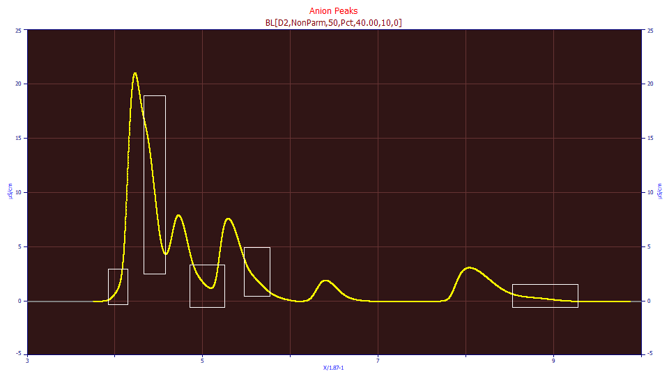
We will borrow an example from the Fitting
Hidden Peaks tutorial.

When the solutes elute closely together, as in the example above illustrating five hidden peaks and three appreciably overlapping local maxima peaks, the analysis need not call into play a monumental effort to change columns, prep, introduce gradient procedures, etc., in order to realize baseline-resolved components for conventional instrumental analysis. At times, one may wish to simply know how many components are present in the data. As a further step, one may want to estimate the quantity and retention times for each of the components. All of that is possible with non-linear peak fitting. With some experience in the analytical modeling of these peaks, that information is readily and swiftly attainable.
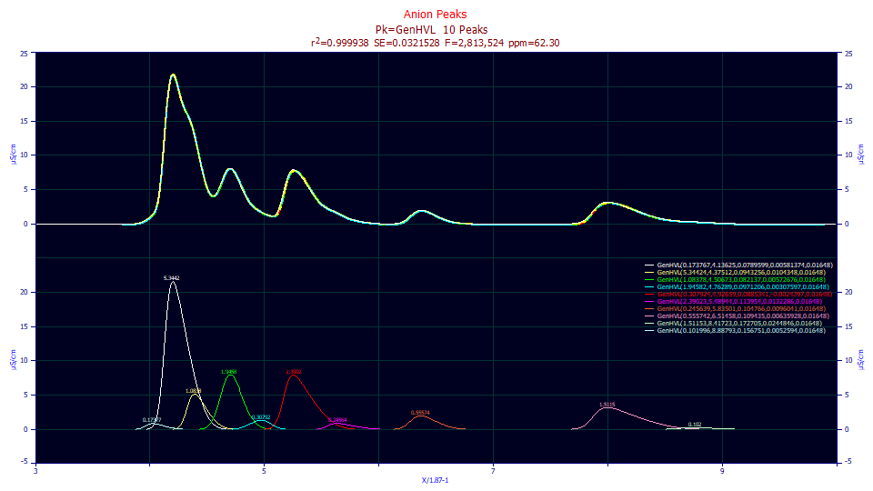
Once you have characterized the IRF of the instrument/column/prep for the analysis, using good standards, the instrument response can be removed from data as muddled as the example above in mere seconds. Then, with the proper use of nonlinear fitting, the components, quantities, and retention times can be realized nearly as swiftly. The information that would be realized from hours, days, or even weeks, of refining the separation can be achieved from the original separation with the overlapping and hidden peaks. In this example, data are sampled to a very high precision, a very good S/N, but the components are simply too similar to elute independently.
Data can still be of an exceptional quality even when baseline-resolved peaks are not present. For this data, the component peaks are estimated to 62 ppm least-squares error, exceptional given the complexity of the fitting problem. Further, as a consequence of non-linear fitting being an advanced statistical procedure, there are confidence statistics which specify how accurately these overlapping and hidden peaks are estimated. A conventional instrument integration would report five peaks instead of ten, and even then the areas of the three overlapping peaks would be inaccurate arising from the intersecting tangent procedure routinely used to assign the area associated with a single point in an overlapped region to one specific peak.
Parametric Modeling a1 - a True Center of Mass
When fitting a chromatographic peak to a mathematical model, you are performing a true parametric estimation. Each of the fitted parameters will tell you something meaningful and important in your analysis. Although we covered the quantity and retention locations in the above example, we will go a step further in looking at the differences between parametric retention times versus that of the mode or peak apex locations typically given in conventional integration procedures.
In PeakLab, the default generalized models report the center of mass of the zero-distortion (infinite dilution) peak minus instrumental effects fitted, but allowing for a multiple-site adsorption third moment adjustment in this zero-distortion density (ZDD). PeakLab also offers [Z] density models which report the ZDD center of mass which would exist if only a single site adsorption were present. This parametric approach offers estimates of retention times significantly more meaningful than simply reporting the apex location of the peak.
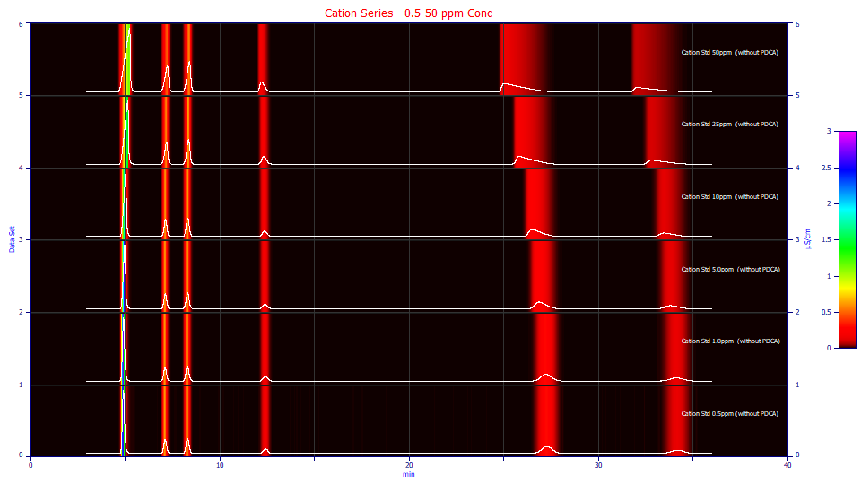
Here we are looking at six cation standard data sets (each with six peaks) similar to the non-additive samples used in the second tutorial. In this example, no additive is present to hasten the retention times. The concentrations vary from 0.5 ppm to 50 ppm across the six samples. The 0.5 ppm sample has barely enough S/N to support a peak fit. At the 50 ppm sample, a small measure of column overload is present.
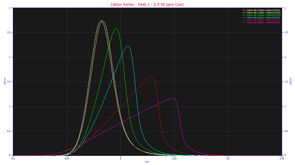
If we look at the first eluting peak with an area normalization across the six concentrations, we see this increase in concentration producing sharply stronger fronted shapes and immense differences in the peak apex location.
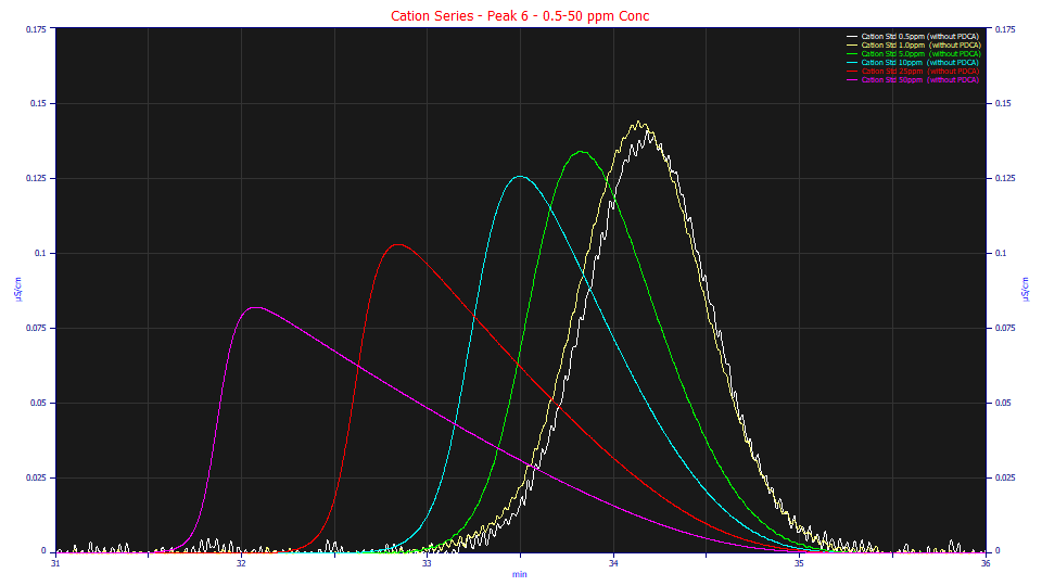
Similarly, if we look at the last eluting peak, we see the increase in concentration producing sharply stronger tailed shapes, and again considerable differences in peak apex location. The S/N on the lower concentration samples is especially evident.
Would it be useful to have a retention value that wasn't all over the map with differences in a solute's concentration? This is possible with nonlinear modeling. The first item to note is that the peaks, as eluted, do have dramatically different centers of mass. To see much closer to a constant center of mass at different concentrations, two items are needed, both of which nonlinear peak fitting can provide. First, the instrumental distortions must be removed or deconvolved. More importantly for this a1 retention value, the impact of concentration on peak shape, as shown above, must be deconvolved in the fitting.
If we fit the GenHVL model to the six different concentration data sets, we see the following retention values:
|
|
Apex Locations |
|
|
|
|
|
|
GenHVL a1 |
|
|
|
|
|
|
Peak |
0.5 ppm |
1 ppm |
5 ppm |
10 ppm |
25 ppm |
50 ppm |
|
0.5 ppm |
1 ppm |
5 ppm |
10 ppm |
25 ppm |
50 ppm |
|
1 |
4.91 |
4.92 |
4.98 |
5.03 |
5.14 |
5.24 |
|
4.89 |
4.87 |
4.87 |
4.85 |
4.81 |
4.75 |
|
2 |
7.12 |
7.12 |
7.13 |
7.14 |
7.19 |
7.24 |
|
7.10 |
7.08 |
7.09 |
7.09 |
7.07 |
7.03 |
|
3 |
8.30 |
8.29 |
8.30 |
8.31 |
8.36 |
8.40 |
|
8.28 |
8.26 |
8.28 |
8.27 |
8.27 |
8.23 |
|
4 |
12.43 |
12.41 |
12.39 |
12.36 |
12.32 |
12.21 |
|
12.40 |
12.39 |
12.40 |
12.39 |
12.41 |
12.40 |
|
5 |
27.28 |
27.23 |
26.87 |
26.51 |
25.83 |
25.05 |
|
27.34 |
27.30 |
27.31 |
27.30 |
27.29 |
27.21 |
|
6 |
34.18 |
34.14 |
33.83 |
33.50 |
32.85 |
32.08 |
|
34.21 |
34.16 |
34.19 |
34.19 |
34.23 |
34.22 |
Which would you prefer to use in order to infer whether or not a retention difference was real, or a concentration effect? The apex locations are the modes of the peaks as eluted. The a1 values are the center of mass fitted parameters in the GenHVL model for these same peaks. For the first three peaks, the fronted ones, the reduction in differences across concentration is 50-60%. For the last three peaks, the tailed ones, the reduction is an impressive 89-97%.
How often have you made a change in a prep or column where both the measured area and retention changed, and you wished to infer a simple direction as to whether or not that change was beneficial? With an accurate parametric model, you can have very close to a concentration-independent estimate of the first moment, the center of mass of the peak that would exist at infinite dilution.
Parametric Modeling a2 - a True Measure of Broadening
In PeakLab, the a2 width in a chromatographic model is reported as either a statistical diffusion width (following the HVL model) or as a first order kinetic time constant (following the NLC model). In conventional analysis, you typically see a FWHM, a full-width at half-maximum, the width of the eluted peak at 50% of the peak's height.
If we look at the fit of the GenHVL model to the six different concentration data sets, and look at the FWHM and a2 SD values for the six peaks across the six concentrations, we see the following:
|
|
FWHM |
|
|
|
|
|
|
GenHVL a2 |
|
|
|
|
|
|
Peak |
0.5 ppm |
1 ppm |
5 ppm |
10 ppm |
25 ppm |
50 ppm |
|
0.5 ppm |
1 ppm |
5 ppm |
10 ppm |
25 ppm |
50 ppm |
|
1 |
0.124 |
0.124 |
0.132 |
0.155 |
0.223 |
0.316 |
|
0.048 |
0.047 |
0.048 |
0.048 |
0.051 |
0.057 |
|
2 |
0.164 |
0.165 |
0.166 |
0.167 |
0.178 |
0.209 |
|
0.064 |
0.065 |
0.066 |
0.066 |
0.068 |
0.072 |
|
3 |
0.182 |
0.182 |
0.182 |
0.182 |
0.187 |
0.211 |
|
0.071 |
0.072 |
0.073 |
0.073 |
0.073 |
0.077 |
|
4 |
0.276 |
0.277 |
0.278 |
0.279 |
0.285 |
0.299 |
|
0.112 |
0.113 |
0.114 |
0.114 |
0.115 |
0.116 |
|
5 |
0.644 |
0.645 |
0.682 |
0.758 |
0.976 |
1.237 |
|
0.266 |
0.269 |
0.275 |
0.280 |
0.292 |
0.311 |
|
6 |
0.793 |
0.809 |
0.812 |
0.868 |
1.063 |
1.334 |
|
0.332 |
0.341 |
0.338 |
0.346 |
0.361 |
0.385 |
Clearly, the peaks sharply broaden with retention time irrespective of concentration.
If we look only at concentration, the FWHM values suggest anywhere from a 1.7-2.5x increase in broadening as the six peaks span the two orders of magnitude concentration. On the other hand, the a2 diffusion width of the GenHVL model increases by just 1.04-1.20x. If you wished to infer anything associated with the measure of broadening in a peak, which of these two values would you wish to use? Unlike the FWHM, the a2 diffusion or kinetic width will be independent of the concentration's impact on the peak shape.
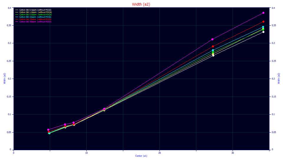
If we plot the the a2 SD diffusion width against the a1 center of mass in the GenHVL fits, we see that the first four concentrations overlap at early retentions and only diverge at extended elution times. The 25 ppm concentration is slightly above the lower concentration curves, and the a2 for the 50 ppm sample is higher still, suggesting a very small measure of overload in the 25 ppm sample, and a somewhat higher measure of overload in the 50 ppm sample. Wouldn't it be useful to see where an analytic overload begins to occur within a column and how that threshold changes as the column ages?
Parametric Modeling a3 - an Absolute and Normalized Measure of Fronting or Tailing
Peak fitting addresses the fact concentration increases the intrinsic fronting or tailing, the a3 chromatographic distortion. We note that the GenHVL and GenNLC models have a common a3 distortion parameter. Since the distortion is a function of concentration, the normalized a3/a0 value is a measure of the intrinsic fronting or tailing in a peak irrespective of concentration.
A fronted peak has a negative a3, a tailed peak a positive a3. With conventional integration, you will generally see only a half-height asymmetry. In a parametric fit, you estimate a parameter that directly estimates the measure of fronting or tailing, and it can be the actual measure of such as influenced by concentration, or it can be a normalized area-independent value:
|
|
Aysm50 |
|
|
|
|
GenHVL a3/a0 |
|
|
|
|
Peak |
5 ppm |
10 ppm |
25 ppm |
50 ppm |
|
5 ppm |
10 ppm |
25 ppm |
50 ppm |
|
1 |
0.563 |
0.375 |
0.213 |
0.143 |
|
-0.00119 |
-0.00115 |
-0.00113 |
-0.00112 |
|
2 |
0.951 |
0.868 |
0.667 |
0.482 |
|
-0.00088 |
-0.00080 |
-0.00080 |
-0.00082 |
|
3 |
0.988 |
0.938 |
0.777 |
0.575 |
|
-0.00048 |
-0.00042 |
-0.00044 |
-0.00050 |
|
4 |
1.082 |
1.158 |
1.387 |
1.747 |
|
0.00102 |
0.00134 |
0.00150 |
0.00146 |
|
5 |
1.710 |
2.453 |
4.287 |
6.313 |
|
0.00985 |
0.01000 |
0.01003 |
0.00995 |
|
6 |
1.438 |
1.922 |
3.292 |
5.015 |
|
0.01327 |
0.01368 |
0.01409 |
0.01424 |
Here we are in the domain of the third moment, and the 0.5 and 1 ppm samples have too little intrinsic skewness and too weak a S/N to fit to full significance. We thus look only at the 5-50 ppm concentration samples. Here we have normalized a3 by the a0 area since parametric modeling offers the means to estimate a concentration-indepedent fronting or tailing. We again ask a similar question. If you wished to characterize the shape of a chromatographic standard and watch for column health or other changes, which of these two metrics would you choose to use?
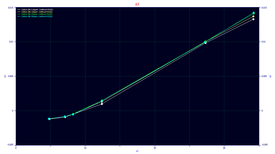
For this plot, we fit a user-defined peak where a3 was the normalized rather than the absolute chromatographic distortion. The dramatic progression from fronted to tailed is apparent at all four concentrations, as is the close to constant normalized a3 distortion for each of the six peaks in the standard.
Parametric Modeling - the Higher Moment Chromatographic Parameters
The a0-a3 chromatographic parameters have a long and well-founded history. The HVL model was published more than a half-century ago and the NLC more than a quarter-century ago. We consider these two models the core diffusion and kinetic models of chromatography. Across these decades, parametric modeling with the HVL and NLC did not present the highly accurate estimations you see in the GenHVL and GenNLC models in PeakLab. The HVL and NLC models, as published, did not include an instrument response component, nor did they include a third moment infinite dilution adjustment accounting multiple adsorption sites. There was certainly no fourth moment adjustment for the dilation occurring in the overload or preparatory shapes, or for the compression occurring in gradient HPLC shapes.
In effect, there were no higher moment adjustments of the ZDD or infinite dilution density in the HVL and NLC models. The HVL assumes a Gaussian ZDD with its zero skewness third moment. The NLC assumes a Giddings ZDD with its fixed location-dependent skewness. No one could actually know just how good the HVL and NLC science happened to be until an effective IRF was added to the fitting, and a third-moment adjustment was added to account multiple-site adsorption or any other non-ideality directly impacting the actual chromatographic separation.
The GenHVL and GenNLC a4 - an Estimate of Multiple-Site Adsorption
Unique to the generalized PeakLab once-generalized chromatographic models, there is an a4 parameter which adjusts the asymmetry of the infinite dilution density (ZDD). This a4 parameter is thought to adjust for multiple site adsorptions, since the skewness adjustment is consistently greater than that which is predicted by single-site NLC theory. The a4 parameter in the GenHVL and GenNLC models is a general third moment adjustment which addresses all non-idealities in the core HVL and NLC models. It uses a statistical generalization of the normal density. The GenHVL and GenNLC models fit any peak identically, including exact fits to the pure HVL and NLC shapes. The difference between the GenHVL and GenNLC rests solely in the GenHVL reporting diffusion-theory parameters, and the GenNLC reporting kinetic-theory parameters. In effect, PeakLab offers one universal chromatographic model with two very distinct parameterizations. Since the two models are equivalent apart from the specifics of parameterization, PeakLab can optionally report the parameters for both models, even when only one is fitted.
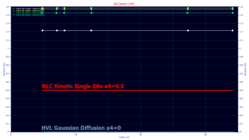
Unlike the core chromatographic parameters, the third moment ZDD adjustment, a4 in the GenHVL and GenNLC models, is usually shared across all peaks. In the above plot of GenNLC fits to this same data, we have two reference points. A pure symmetric Gaussian ZDD, which produces a pure HVL, occurs at a4=0. A pure Giddings ZDD, which produces the NLC, occurs at a4=0.5. The GenNLC, as a kinetic parameterization, is indexed to the Giddings/NLC. The value shown in this plot is typical of what you will likely see in PeakLab. The Giddings-indexed ZDD asymmetry in this example is 2-3x higher than predicted by the single-site NLC kinetic theory.
With this parameter we address the deviation from HVL and NLC theory in the actual chromatographic separation. Since this is also an adjustment which impacts the third moment, these a4 estimates will be more accurate at higher concentrations. The a3 chromatographic distortion acts upon this ZDD; the more a peak is tailed or fronted, the more this deviation from the theoretical ZDD is reflected in the resultant shape of the peak.
If we fit a GenNLC and lock the a4 value at 0, we fit pure HVLs. If we lock that a4 value at 0.5, we fit pure NLCs. If we allow a4 to be adjustable, we will typically fit a peak whose shape whose ZDD is appreciably more right skewed than the NLC's Giddings density.
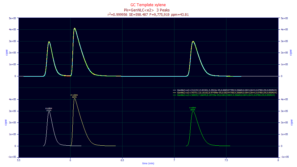
Because the HVL was developed primarily for GC, we initially expected to see a4 values in GC data close to zero, the theoretical HVL. The above fit is from the data used in the IRF Estimation - GC topic. For this GenNLC<e2> fit, the a4 shared across the three isomer peaks is 9.21!
If a4 is an estimate of the aggressiveness of the binding at least with respect to capturing additional adsorptions, it should be especially useful for characterizing changes in column health or subtle changes in solutes which don't alter areas or retention times but produce higher moment differences. You may wish to refer to the HPLC Column Health and Overload tutorial.
The Gen2HVL and Gen2NLC a4 and a5 - Third and Fourth Moment Adjustments
PeakLab's twice-generalized models adjust both the third and fourth moments of the ZDD. In these models a4 is the power of decay in the tailing, impacting the fourth moment or kurtosis of the peak, and a5 is the asymmetry adjustment impacting the skewness or third moment. This is realized by using a generalized error model for the ZDD.
These more complex models are mostly used for preparative shapes with high overload, where a dilation occurs in time, and for direct fits of gradient HPLC shapes, where a compression occurs. For most analytical peaks, however, a decay power of 2 Gaussian type of exp(-z2) tailing will be observed and a once-generalized GenHVL or GenNLC with just one higher moment ZDD adjustable parameter is all that is needed.
You may wish to refer to the HPLC Gradient Peaks - Direct Closed Form Fits and Fitting Preparative (Overload) Peaks tutorials as well as the HPLC Gradient Peaks - Direct Closed-Form Fits topic.
The <ge>, <e2>, and <pe> Instrument Response Functions
An immense part of PeakLab's technology rests in the fitting of IRFs or instrument response functions. This is the component of a chromatographic model that describes everything that is not part of the primary chromatographic separation. An IRF includes all delays and distortions arising from the non-idealities in the injection, flow path, detector, and mass transfer resistances with respect to the particles in the column. The mathematical description of this instrumental distortion is a convolution integral, one that PeakLab addresses with a fast Fourier domain fitting. Otherwise minutes become an overnight process.
You can think of the primary chromatographic component of the model as the separation that occurs at the interface between the mobile and stationary phases. You can think of the IRF as everything else that distorts the peak, but which is nowhere associated with that which occurs between the two phases.
In fitting an IRF, there are practical fitting considerations. If there are multiple processes that impact these distortions, it will not be possible to fit a sum of all of them and achieve statistical significance in the fitting. In PeakLab, we can fit one slow component, a high time constant exponential which we describe as a 'system' component of the IRF because it is observed to be nearly constant, independent of process variables. We can also fit one fast component, which we describe as a 'process' component, which sums with the slow component. This fast IRF component is sensitive to process variables such as concentration, temperature, additive levels, and so forth. In practical terms this fast component must address any small mixing delays in the flow system, axial dispersion, and mass transfer into and out of porous particles in the media.
We have three IRFs we use almost exclusively. All three use a first order exponential for the slow system component. This slow component significantly impacts the tailing of peaks as registered by the instrument. Since the fast component is close to an impulse of a much narrower width, its impact on the overall peak shape is small, despite it typically consisting of better than half of the overall quantity of instrumental distortion. We can thus use the <ge> IRF where the narrow component is assumed to be a half-Gaussian modeling the axial dispersion, or the <e2> where the narrow component is assumed to also be a first order exponential, or the <pe> IRF which uses a 1.5 power kinetic to approximate mass transfer resistances in very small media particles where there is a second order step in the overall transport.
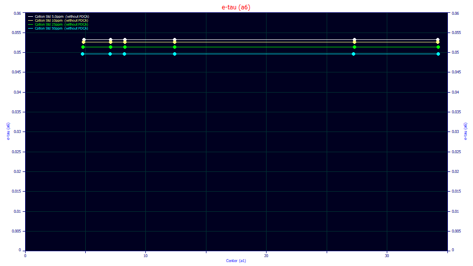
In this six peak cation standard example, the above plot is for a6, the slow exponential tau or time constant, the 'e' component in the <ge> IRF. The differences across the four higher concentrations are quite small, and these do track with concentration. If we assume this slow component of the IRF is mostly associated with the detector, we must conclude that higher concentrations are sensed ever so slightly more swiftly.
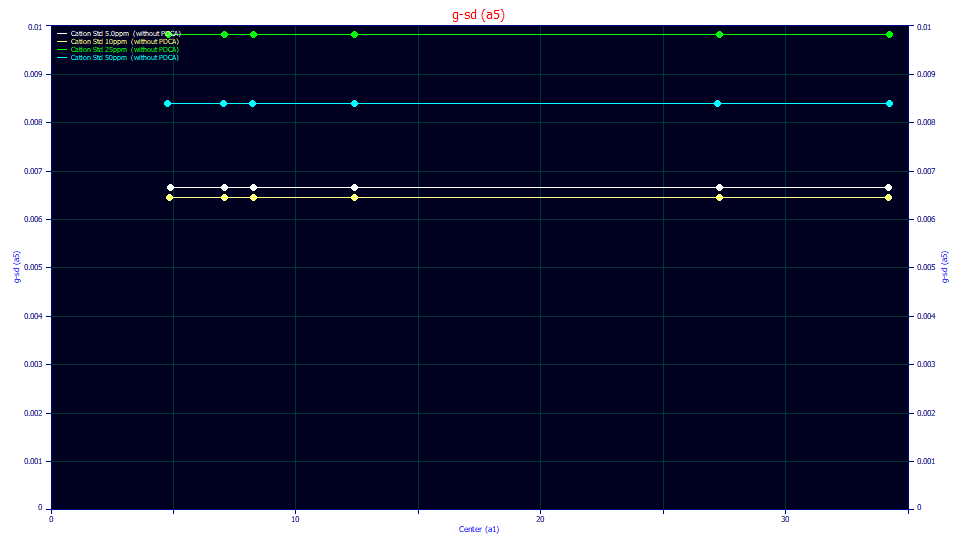
In the above plot, we see a5, the 'g' component in the <ge> IRF, where the narrow component is treated as axial dispersion and fitted to a half-Gaussian. This narrow width component has a half-Gaussian SD that is only 5-10% of the exponential time constant in the slow component. The a5 parameter does vary more, and it does not track concentration, but we also know this component is the least significant of those fitted, even though some form of narrow width component is absolutely essential for an effective IRF.
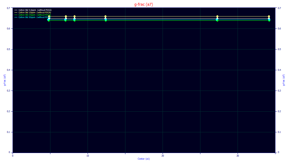
This is a7, the fraction of the overall area of the IRF assigned to the narrow component. Here we see this close-to-impulse component of the IRF consisting of close to 2/3 of the overall distortion. For the data we've worked with, this fraction of components is also close to constant across process variables.
It is also worth noting that the IRF parameters can actually be used to map overload in preparative peak modeling.
In fitting a GenHVL or GenNLC model to chromatographic data, you should see the a0-a4 parameters in light of column health. You should see the IRF a5-a7 parameters as indicative of the state of the instrument's health, as it specifically addressing the state of the flow path, detector, and the measure of all of the different factors that enter into this narrow width IRF component. For example, if the pores of the media are beginning to close off, this narrow width component would be expected to widen, whether it is being fitted as Half-Gaussians ('g'), a first order kinetic ('e'), or 3/2 power kinetic ('p').
We generally fit the <ge> IRF since the two components are least correlated. You may wish to refer to the IRF Model Fits topic for a comparison of these three principal IRFs. There is a large body of information in the help system and tutorials to help you better understand how to estimate and use IRFs effectively in PeakLab.
An Immense Improvement in Fit Quality
It is also worth noting that in the examples, we fit six peaks with a0-a3 core parameters, a total of 24 parameters. With the four a4-a7 parameters shared across the peaks, the overall fits each consisted of 28 parameters. The one shared ZDD parameter and three shared IRF parameters are necessary to extract meaningful information for column and instrument health and to better understand the chromatographic process. The difference between including the four additional parameters and omitting them is day and night with respect to the peak fit. Without these parameters, the least-squares fitting error is between 3000-4000 ppm, something we once believed to be quite good. With these four parameters, the four higher S/N data sets in these examples fit to less than 20 ppm error; three fit to less than 10 ppm.