PeakLab v2 Documentation Contents R2N Software Home R2N Software Support
Modeling Spectra Tutorial II - Powder FTNIR
In this second modeling tutorial, we will generate certain of the models documented in the Modeling Spectra - Part II - FTNIR Data white paper.
You may wish to first explore the first modeling tutorial, Modeling Spectra Tutorial - Liquid UV-VIS, if you have not already done so. It covers many of the basics of direct spectral modeling.
Where as the the Modeling Spectra - Part II - FTNIR Data white paper focuses on many of the intricacies of FTNIR spectral modeling, this tutorial will focus on maximizing the accuracy and robustness when selecting a spectral model.
FTNIR Spectral Modeling
In this tutorial, we will demonstrate the much more challenging FTNIR spectral modeling of powders. We will estimate the total curcuminoids in turmeric powders.
By directly analyzing the powders, we will see a much more complex modeling problem. The reflectance of powders is impacted by both powder particle size and powder moisture levels. The particle size density will vary across the turmeric samples as a consequence of processing, and the NIR spectra for a given turmeric will vary with the moisture (there are two prominent water bands in the NIR).
FTNIR Spectroscopy of Curcumin vs Turmeric - Obfuscating Absorbances
In the Modeling Spectra - Part II - FTNIR Data white paper, we illustrate the rather staggering differences between the curcuminoid FTNIR spectra and that of the turmeric powders which are known to consist of many different molecules, some having NIR absorbances that compete with the two principal bands used for curcuminoid analysis. In this tutorial will we exclusively fit the 1650-1850 nm NIR band.

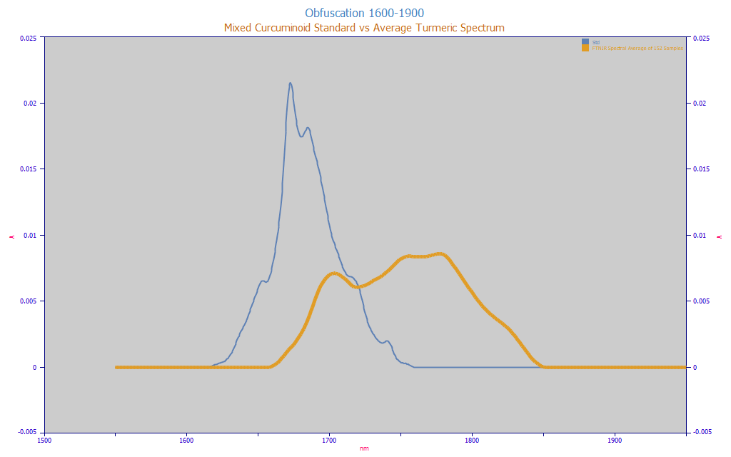
Fig. 1 Obfuscation of Curcuminoid Target Spectrum in Natural Turmeric (average spectrum from 146 turmeric samples), 1600-1850 nm, Equal Area
In Fig. 1, we repeat the plot from the white paper of the obfuscation of the curcuminoid spectra within the turmeric powders. The blue spectrum is for a curcuminoid standard. The amber curve is the average FTNIR spectrum from 146 different turmeric samples.
Powder vs. Liquid Spectra
We expect this NIR modeling to be much more challenging than the UV-VIS of Part I. We have these obfuscating absorbances in the modeling bands. Turmeric, a natural agricultural product, is known to contain a very large number of components (some authors have reported up to two hundred) and its curcuminoid content and fractions can vary immensely from one sample to the next. The average curcuminoid content is only about 4% of the overall solids in a turmeric powder. On average, 96% of the turmeric solids are non-curcuminoid. Further, all that a compound within the turmeric needs to appear within this 1650-1850 modeling band is a C-H bond. The additional absorbances of non-curcuminoids in the modeling bands are thus not surprising.
In the Modeling Spectra - Part II - FTNIR Data white paper we extensively cover the many other challenges that exist in extracting quantitative information from NIR reflectance powder spectra.
For this modeling, we know we have non-curcuminoid spectral information that will impact the absorbances. We also know that even with basic sieving to remove the larger particles, there can be significant differences in spectral magnitudes of samples that appear virtually identical in the HPLC. Two turmeric samples with with essentially identical curcuminoid chromatography can have very different spectra as a consequence of the optics of powder reflectance as well as non-curcuminoid content. We also have concerns with the nonlinearity of the powder spectra with moisture content.
Resolution and S/N of FTNIR Spectra
In the In the Modeling Spectra - Part II - FTNIR Data white paper, we estimated a Gaussian SD for the curcuminoid standard in FTNIR spectra at 3.6 nm, an exceptional resolution. In the Fourier Estimation of Spectroscopic Resolution topic, we confirm that estimated resolution in a Fourier domain procedure.
We also tested the S/N of individual FTNIR turmeric spectra using the DSP menu's Fourier S/N Estimation and we see an exceptional 0.020-0.025 % estimated white noise in these spectra.
In the Modeling Spectra - Part II - FTNIR Data white paper we explain our rationale for using a 2 nm spacing in our direct spectral fits to this FTNIR data.
Direct Spectral Fit
From the Model menu's Import Data Matrix item, select the Import Spectroscopic Data Matrix... option. Select the data matrix file ModelingFTNIR_SpectralData.csv from the program's installed default data directory (\PeakLab\Data). Answer No when asked if you wish to proceed to fit this data.
From the Model menu's Graph Data Matrix item, select the Graph All Data Sets in Spectroscopic Data Matrix... option. Select 1650 for the starting X-column and 1850 for the ending X-column and click OK.
In the identification portion of the dialog, enter pctTotal:4 as the search string and click Find. This will highlight all of the data in the file where this substring appears in the data set identification column(s). In this example, all spectra are highlighted where the total % curcuminoid ranges from 4.00 to 4.99 %:
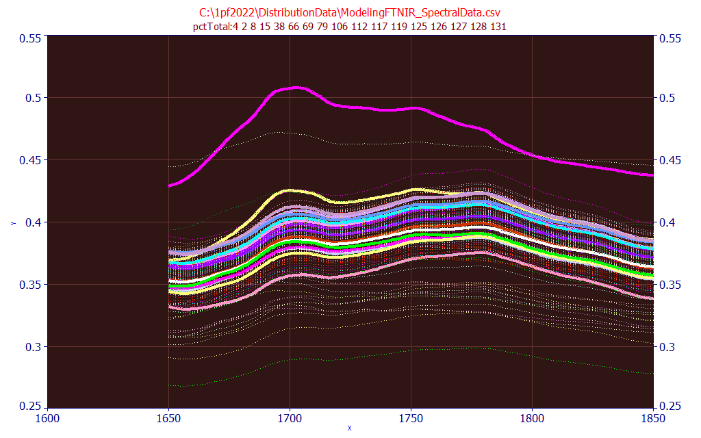
Fig. 2 FTNIR Powder Spectra with total curcuminoids 4.00-4.99 highlighted
As you will note, this is not a simple modeling problem. The total percentages vary from near 0 to very 14% in the above set of spectra, and there is no wavelength in the NIR where there is not a wide range in spectral magnitudes for this 4-5% band that is highlighted. Click the different normalizations None, Unit Area, Unit Magnitude, Zero Mean, and Mn=0 SD=1 to see if any of these result in these 4-5% samples converging to a narrow band in the set if spectra. You should be able to fairly swiftly confirm that this will be a multivariate modeling problem that will consist of some number of wavelengths as the independent variables. Click OK to close.
Once the Import Data Matrix | Import Spectroscopic Data Matrix... item in the Model menu is used to load a spectroscopic modeling data matrix into the program, the Fit GLM Models option is available for fitting full-permutation GLM models, smart stepwise forward models, and sparse PLS models, the latter two each using the full permutation models as their starting point.
The PeakLab full permutation GLM models are a simpler and more affective alternative to the PLS (partial least squares) and PCR (principal component regression) procedures.
From the Model menu, select the the Fit Full Permutation GLM Models... option. This is the entry point for all predictive modeling.
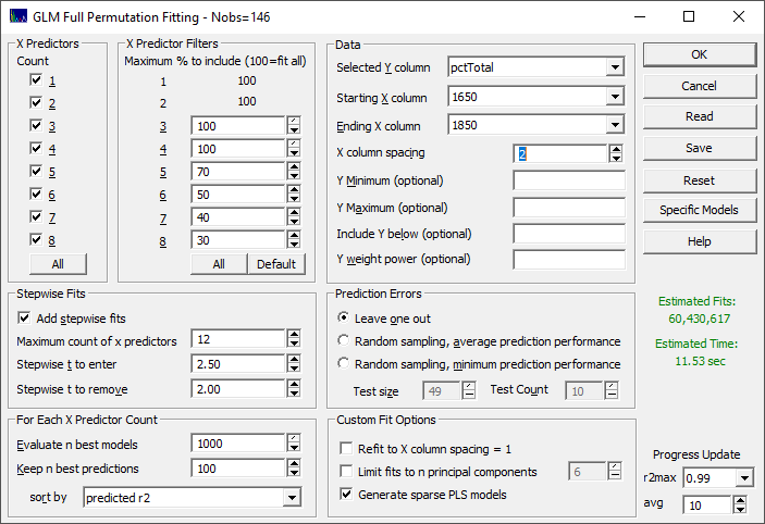
Fig 3A. The fit specification for the initial fitting of the turmeric spectra
There are seven sections that govern the modeling.
X Predictors
We want to fit all of the X-predictors through the full eight allowed in the GLM full permutation algorithm. Click All in the X Predictors section to select all of the predictor counts if needed.
X Predictor Filters
Because we will be using such a small X column spacing (2 nm), we wisely use the default filters to thin the wavelengths fitted as the parameter count increases. Click Default so that the filtering is shown as above.
Stepwise Fits
We will use the defaults. Be sure Add stepwise fits is checked, the Maximum count of x predictors is set to 12, the Stepwise t to enter is 2.50, and the Stepwise t to remove is 2.00.
For Each X Predictor Count
We will also use the defaults. Be sure Evaluate n best models is set to 1000, Keep n best predictions is 100, and the sort by is set to predicted r2. These numbers specify retaining the best 1000 models (by least squares error in the model fits) at each predictor count, evaluating them for the best r2 of prediction, and keeping 100 models for the GLM Review.
Data
Select the pctTotal column in the data file for the Selected Y column, 1650 as the Starting X column, and 1850 as the Ending X column. Enter 2 for the X column spacing. You should see, in green, a fitting time less than 1 minute. We will begin the fitting with 101 parameters, the spectral values from 1650 to 1850 at an increment of 2 nm. The estimate should reflect that 60 million actual models will be fitted.
Prediction Errors
Be sure the Leave One Out is selected.
Custom Fit Options
Leave the Refit to X column spacing = 1 unchecked. The 2 nm resolution will be sufficient.
Click OK to start the fitting.
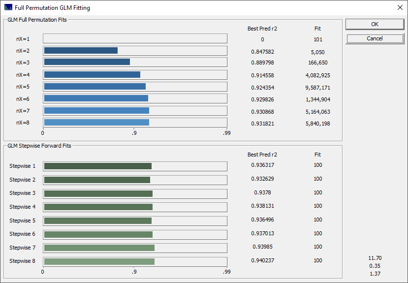
Fig 3B. The r� progression in the fitting, each bar represents an average of the 10 best models of that predictor count
If you did the UV-VIS of Part I tutorial, you saw a very different outcome from fitting the liquid UV-VIS spectra of the samples solubilized in the chromatography's mobile phase. In the liquid UV-VIS case of total curcuminoid content modeling, there were no competing absorbances and there were no powder measurement issues.
Click OK when the fitting is done. Accept the default file name and Save the full fit information to disk. By subsequently importing this file using the Model menu's Import GLM Models for Review... item, you can recall these fits in a single step.
Reviewing the Direct Spectral Fits
You will now see the GLM Review. The GLM Review assembles the full-permutation GLM models, the smart stepwise forward models, and the sparse PLS models for an intelligent selection of a final predictive model.
The two most important windows will be the Model List window and the main GLM Review window containing the model plot and significance map.
Finding the Optimal Count of Predictors (wavelengths)
The first step in the process, however, will usually be the determination of the optimum parameter count. Click the Fit Performance button.
![]() From the window containing the graphs of the fit metrics, click the Toggle Display of
Reference Data in the toolbar. This will disable the reference data in the plot which contains the
model fit statistics. We will look only at the prediction statistics.
From the window containing the graphs of the fit metrics, click the Toggle Display of
Reference Data in the toolbar. This will disable the reference data in the plot which contains the
model fit statistics. We will look only at the prediction statistics.
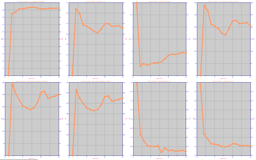
Fig. 4 The prediction statistics as a function of predictor count
Although we want to see where the SE of prediction is at its best (second panel, 8 WLs), we prefer to look at the information criteria, the Akaike AICc (fourth panel, 8 WLs), the Bayesian BIC (fifth panel, 7 WLs) and the Minimum Description Length MDL (sixth panel, 7 WLs). The average absolute prediction error is also useful (eighth panel, 8 WLs). The metrics are consistent in suggesting that a 7 predictor or 8 predictor model is going to be needed for the best prediction performance.
Click OK to close the fit performance window.
Limiting the Models to Only those of Interest
In the Model List's Filter menu, select the Include 7 Predictor Models to limit the list to those with just 7 wavelengths. Also select the Include 8 Predictor Models. The list now contains only models with 7 and 8 wavelengths:
Indx nX Predr2 PredAvErr Model
1 7 0.9411508 0.3023832 Step[7,3](1654,1656,1670,1688,1750,1798,1828)
2 8 0.9409551 0.2956805 Step[8,7](1658,1672,1682,1688,1702,1748,1782,1828)
3 8 0.9408350 0.2994798 Step[8,2](1656,1674,1680,1688,1702,1750,1782,1828)
4 8 0.9408093 0.2953673 Step[8,4](1656,1672,1682,1688,1702,1750,1782,1828)
5 8 0.9405478 0.3041807 Step[8,3](1654,1656,1670,1688,1750,1782,1810,1828)
6 7 0.9402614 0.3019120 Step[7,4](1654,1656,1668,1688,1750,1800,1828)
7 8 0.9402247 0.2964691 Step[8,7](1658,1672,1682,1688,1702,1758,1782,1828)
8 8 0.9401743 0.3061181 Step[8,7](1654,1656,1670,1686,1750,1782,1810,1828)
...
For these data, the best fits, by the 'leave one out' prediction metric, are the stepwise models which begin with various predictor counts of the full permutation fits. For these data, the best overall prediction goodness of fit r� is only going to be about 0.94 as contrasted with the greater than 0.99 observed in the UV-VIS modeling of the same turmeric samples.
If this data matrix is fit to 6-factor, 7-factor, 8-factor, and 9-factor PLS models (NIPALS algorithm), at a 2nm spacing (101 wavelengths), the leave one out Prediction r2 is 0.923, 0.928, 0.926, and 0.925. We have never encountered a spectral data matrix where the PLS or PCR models perform as well for prediction as the better direct spectral fits.
Note that the intelligent stepwise fits do not use the full permutation filters, so even if a WL is omitted from the permutation matrix by a filter, it may still appear within one of PeakLab's stepwise models. Please note that these are not the simple forward stepwise models you may have fitted in statistics software. Each of these "stepwise" models contains a kind of multidimensional search that seeks to find the best models from a given full permutation model starting point. In this different form of algorithm, a WL predictor that is removed from a model can be added back further along in the process. In general, you will see some benefit in these stepwise models that arise from starting with very effective full permutation models. The stepwise algorithm allows models up to 15 predictors to be fit.
Selecting a Model by Best X-Predictor Significance Compliance
The best model in the fitting, by r2 of prediction error, using the leave one out estimate of prediction error, is a 7-predictor model with a r2 of prediction of 0.9412. For our purposes, we will select a 7-predictor model (as suggested by the BIC and MDL information criterion) based upon a sort of the models by compliance with the average of the significance at the different wavelengths.
The premise is that the best retained predictive models of a given predictor count will, in the aggregate, contain a strong picture of the most significant predictors for that predictor count. Please see the X-Predictor Compliance section in the Model List topic for a more detailed explanation of this sort metric. You can also see a 3D significance plot across all predictor counts.
From the Filter menu in the Model List, unselect the Include 8 Predictor Models. From the Sort menu, choose By X-Predictor Compliance. Be sure the first model in the list is selected:
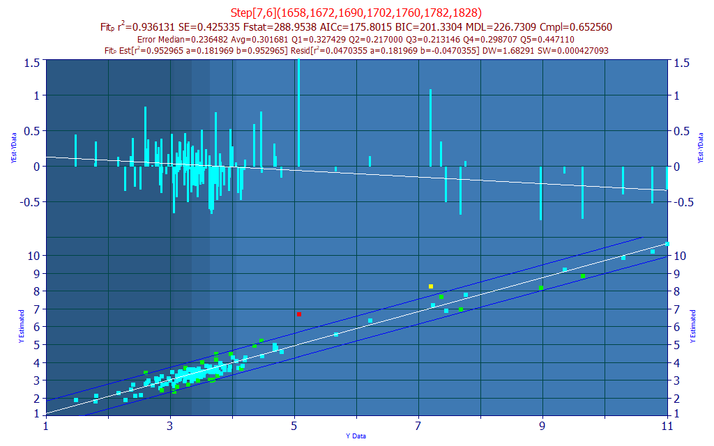
Fig. 5A The selected model plot for the predictive FTNIR model of total curcuminoids
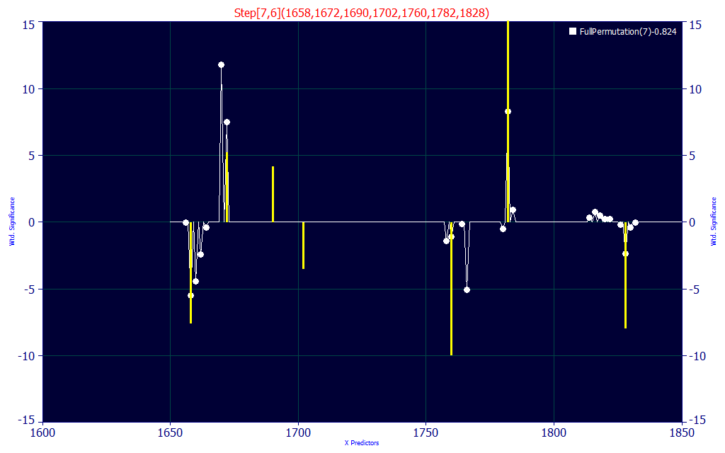
Fig. 5B The selected model and 7-predictor significance plot for the predictive FTNIR model
By requiring the selected fit to consist of highly compliant wavelengths with the retained best 7-predictor count fits, we minimize the possibility of a predictor appearing in the model by random chance.
In the prediction modeling science, one seeks to mitigate the influence of random chance or indirect correlations. A hydrophobic species that is the object of a predictive model, for example, may have an inverse correlation with a hydrophilic species that is also present, but such indirect effects are dangerous in predictions. There may be samples where this additional entity isn't even present, and others where the inverse correlation doesn't apply. You want to have the wavelength band of the species being estimated well represented in the model. In a complex model such as this, where powder moisture, core particle size, and aggregation must also be managed by the model, there will be a mix of positively and negatively correlated spectral wavelengths.
In seeking a model with a high measure of wavelength compliance with the retained best 7-predictor models, we selected a 7-predictor model (Fig. 5A) with an r� of 0.9361 and an average prediction error of 0.3017 % total curcuminoid.
Removing Outliers and Refitting
By visual inspection, there is one prediction that is colored red (>3SE) and one colored yellow (>2SE). These may be outliers that contain an error in the chromatography or spectroscopy. They may as esily be outliers in the samples, quite distinct and apart from all of the other samples in the study. In general, you should manually inspect such samples for the chromatography and spectroscopy replicates to see if the deviation is process related. If not, you should study the chemistry of these samples to learn why of nearly 150 distinct samples, these two could not be effectively modeled. For the purpose of this tutorial, we will assume these two samples are a result of process error. We will treat them as outliers and refit the data with an outlier removal step. Even if we suspect the overall goodness of fit is unlikely to change, it is possible the wavelengths in the best models will follow a certain pattern to keep these two residuals as small as possible. Without that constraint, the wavelength map be more accurate.
Click the Data button to open the GLM Data window. In the Content menu, be sure SE Prediction Intervals is checked. In the Outliers menu, be sure only Flag Outside Prediction Interval is checked and that Prediction Interval Confidence is set to 95 Confidence. You should see '5 Flagged Outliers' in the Data window's title bar.
Highlighted spectra are informational only. The metric producing the highlight state will appear in bold.
Flagged spectra are those which will be removed when the GLM Data window's File menu's Save Data with Flagged Outliers Removed is used. When a spectrum is flagged, all displayed metrics will be grayed and it will be shown with an asterisk.
Use the GLM Data window's File menu's Save Data with Flagged Outliers Removed item and enter the any name and location for the new data file. It will contain 142 spectra instead of 147. The 95% prediction interval criterion resulted in the removal of five of the spectra.
Click OK in the main GLM Review window. From the program's main Model menu, use the Import Data Matrix | Import Spectroscopic Data Matrix and then select the file you just saved with the outliers removed.
From the Model menu, once again select the the Fit Full Permutation GLM Models... option. The options previously set should be present. Click OK to begin the fitting.
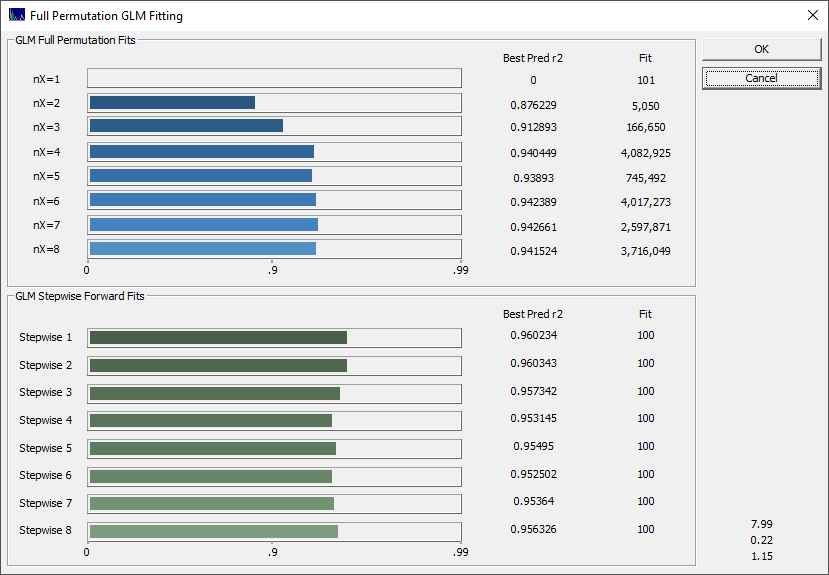
Fig 6. The r� progression in the fitting with the data where the outliers were removed
As you will note, the r2 goodness of fit averages have significantly improved with the removal of these five points we treated as outliers.
Click OK when the fitting is done and specify a file name of your choosing to Save this full fit information to disk.
Selecting a Model by Multiple Criteria
From the Filter menu in the Model List, check Single Predictor Count and then check the Include 7 Predictor Models. In the List menu be sure Avg Error of Prediction, Median Error of Prediction, and XPredictor Compliance are checked. From the Sort menu, choose By Predicted Average Error.
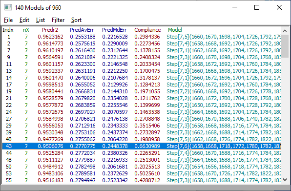
Fig 7. Model list for the data fitted with potential outliers removed
We will choose a model with a good prediction average error and prediction median error, and also one whose WL's are strongly represented in the retained set of 7-predictor models. Select the Model with the Compliance of .66 at index 43 as shown above.
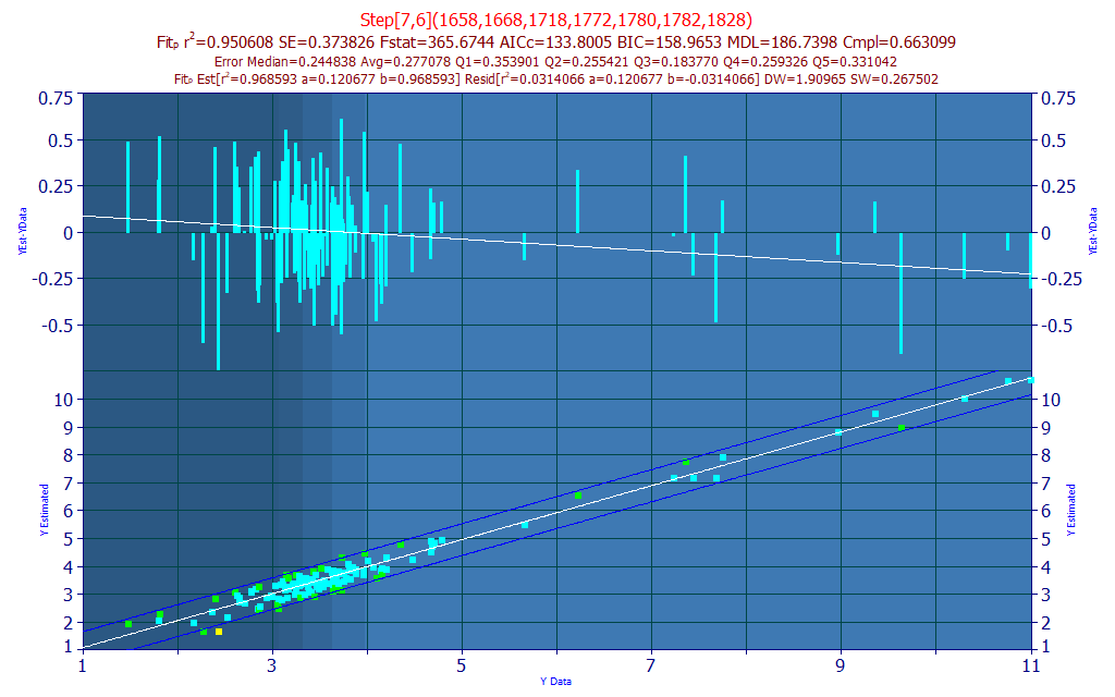
Fig. 8A The model plot for the selected model
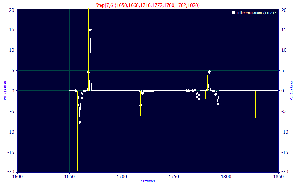
Fig. 8B The 7-predictor significance plot for the chosen model, the model in yellow, the map of all retained 7-predictor models in white
If you look closely at the significance plot, this specific model (in yellow) aligns with many of the WLs in the 100+ retained 7-parameter model averages.
Evaluating a Predictive Model
To this point we have used the built-in 'leave one out' prediction estimates for model selection. In this prediction error approach, all of the samples except the one being predicted are independently fitted and the one withheld sample is processed through that specific set of parameters. The whole of that fit process generates 1 error value. The process is then repeated for the second sample, the third, and so on until there is a set of prediction errors of the same size as the data matrix. This is a good way to test well-bracketed data where the probability of a sample outside the bounds represented in the model data matrix is low.
When working with smaller sample counts where the possibility of a sample being outside the existing bounds represented in the data matrix is high, you can use random sampling errors. This procedure creates random in-sample and out-of-sample data sets of a size and count of sets which you specify, and the errors can be average or worst case. This is how one addresses a predictive model where the model data is insufficient to fully map the expected samples.
In general, you will use the Predict feature to evaluate subsequent data once a model has been implemented.
If you have data that wasn't as rigorously generated (in this example, where an average moisture content was used), or where subsequent chromatography better separated the pertinent components going into a total estimate, those data may be useful for a separate out-of-sample prediction analysis. If the model data consisted of replicate averages that were carefully screened, you may wish to use this feature to see what the predictions would look like if there was no cleansing of the data, or if only a single sample was generated in a field analysis where an average of replicates would not generally be made.
Click the Predict button and select the spectral data matrix file ModelingFTNIR_PredictionData1.csv from the program's installed default data directory (\PeakLab\Data). The is the raw data that with laboratory errors (there were samples errantly mislabeled or swapped) and with all spectral replicates present as individual samples (no average was made).
![]() In the model graph's toolbar, select the Common Scaling for Y and Y2 plots to use a common Y,Y2
autoscaling for the model and prediction plots.
In the model graph's toolbar, select the Common Scaling for Y and Y2 plots to use a common Y,Y2
autoscaling for the model and prediction plots.
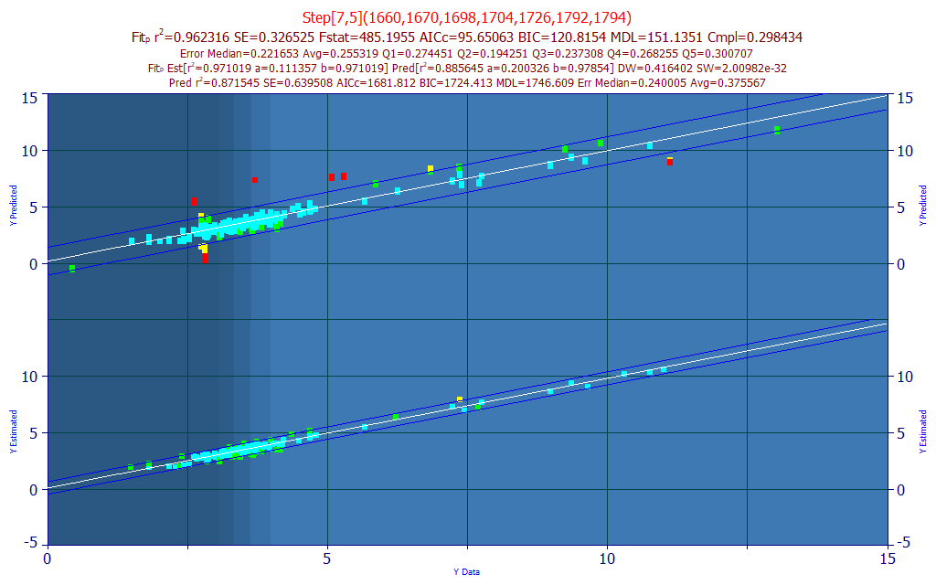
The prediction plot of known vs. predicted is in the upper portion of the graph. Many of these red points are laboratory sample or replicate errors. You should pay close attention when such data are observed. The more accurate the input data, the more accurate the predictive models will be. With these errors in the data, the average prediction error is .375% compared to .255% in the cleaned, averaged data.
Right click the model plot and from the popup menu select Mark Inactive Outside Prediction Interval.
![]() The Confidence
Intervals dialog can be used to change the graph's prediction interval. Be sure to change the Y2 axis
confidence level.
The Confidence
Intervals dialog can be used to change the graph's prediction interval. Be sure to change the Y2 axis
confidence level.
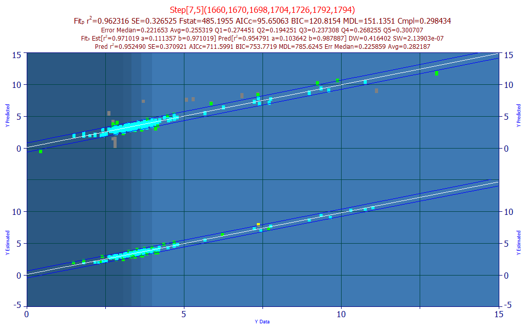
This does an admirable job removing the erroneous spectra from the prediction, while retaining the replicates. If you look at the last line in the title, the prediction average error is .282 with the replicates and .255 with the averages used in the modeling. Roughly comparable, this gives a sense for the degree to which the goodness of fit improves from the averaging.
Click the Prediction button to close the Prediction window and to remove the prediction from the upper portion of the plot.
![]() Note that the common scaling is retained when a prediction is closed. This assumes you may wish to enter
additional sets of prediction data, as we will do. You would again use this Common Scaling for Y and
Y2 plots item in the model graph's toolbar to restore a separate scaling for the residuals plot.
Note that the common scaling is retained when a prediction is closed. This assumes you may wish to enter
additional sets of prediction data, as we will do. You would again use this Common Scaling for Y and
Y2 plots item in the model graph's toolbar to restore a separate scaling for the residuals plot.
Click the Predict button once more and select the spectral data matrix file ModelingFTNIR_PredictionData2.csv from the program's installed default data directory (\PeakLab\Data). The is out-of-sample data done at an earlier time without certain refinements in procedure.
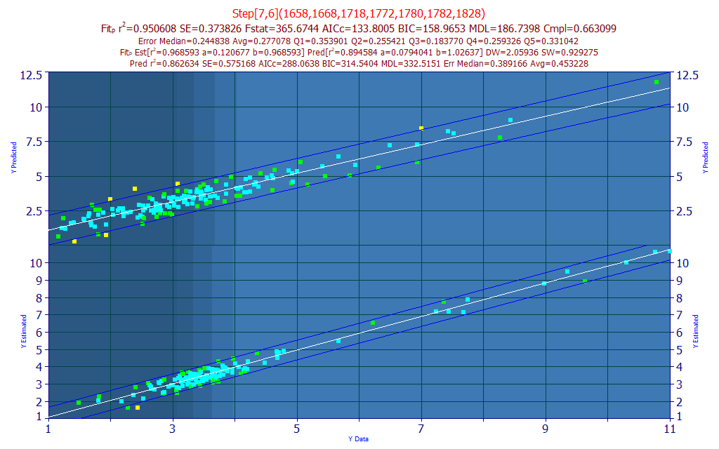
The average prediction error from these data is .453. You will note that the scatter is appreciably higher.
Select the first equation in the list and using the down arrow key, step through the first fifty or so models looking for the lowest prediction error for this prediction data set. You should see none below 0.4 average prediction error.
Robust Predictive Models
One of the benefits of direct spectral fits is that models are far more flexible and far simpler than PLS or PCR models. You can, for example, choose a dozen different predictive models you happen to especially like, implement an average or median of the predicted values from each, and still use less computation than a single evaluation of a PLS or PCR model.
You can also use the quintile errors reported for the models to develop quintile-specific models. One or more models is set for each quintile of Y-values, and an overall model is used to determine which of the quintile-specific models will be used for the prediction. We have realized a reduction in prediction errors on the order of 20% by using this method.
If one of the objectives of the modeling is to produce truly robust predictions, you may wish to explore the convenience of built-in sparse PLS models. With respect to how such models are evaluated, they are similar to PLS and PCR evaluations except that the WL map is sparse; only certain wavelengths are represented. When the Generate Sparse PLS Models option is checked in the fitting dialog, the most significant direct spectral models are integrated into a weighted average prediction that produces a higher count of predictors. In a sparse PLS model, you will see something akin to PLS[15,35,8]. This means that the model consists of 15 predictors (15 wavelengths, 16 estimated coefficients). These will be the 15 most significant predictors in the retained 8-predictor models. This overall model will have been built by the statistical goodness of fit weighting of the 35 direct spectral fits of 8-predictor models which are a subset of these 15 significant wavelengths. You can readily equate the 8 predictor count with a factor count.
In the Model List's Filter menu, check No Filtering and then check Only Stepwise and Sparse PLS Fits. Be sure the Sort is still By Predicted Average Error. Select the first sparse PLS model in the list (you will have to scroll down):
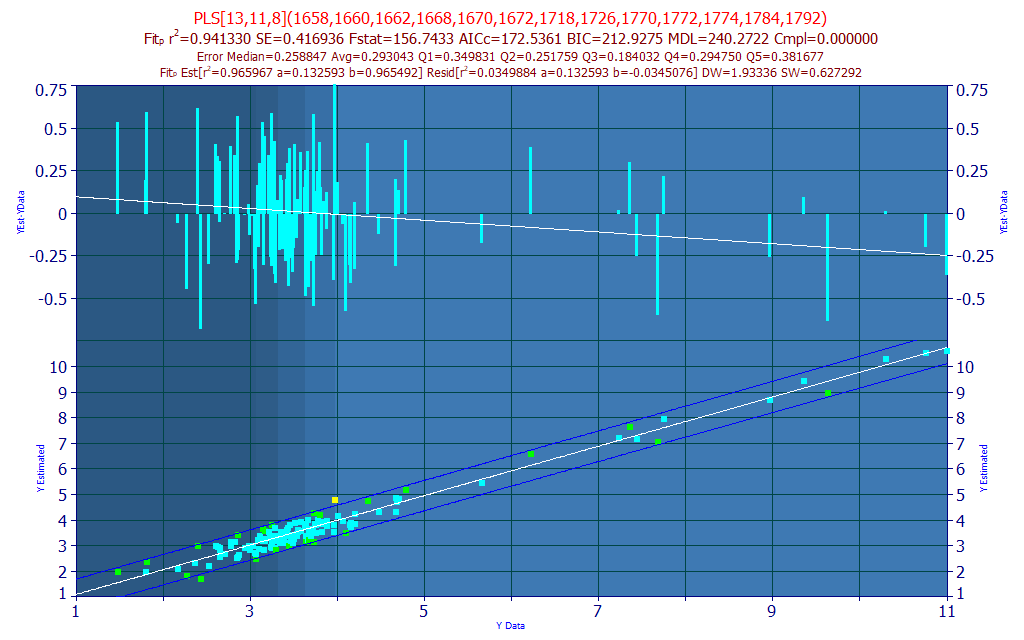
Although the leave one out average predicted error is slightly higher, 0.293 instead of 0.277 for the single model we selected, this model combines 11 very effective 8-predictor models, all of which are subsets of the most significant 13 predictor WLs in the 8-predictor model. In a sparse PLS model, the WLs are not equally represented, but weighted by that WL's significance in the retained models. Certain of the WLs will have higher contributions than others, just as occurs in PLS models.
Implementing a sparse-PLS model, or any of PeakLab's spectral models, is quite easy. Click the Numeric button in the GLM Review window if the Numeric Summary is not presently displayed. In its Options menu, select the first C++ code option. The code is added to the Numeric Summary:
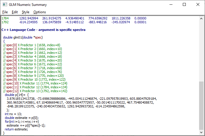
Although the main language export options are C++ and Visual BASIC, the GLM Prediction window also offers Mathematica, Maple, and Excel model export.
Spectral Modeling
As with serious statistical multivariate linear modeling, direct spectral modeling is both art and science. PeakLab furnishes some of the best predictive tools in the industry to ensure your models perform as well as the modeling data permits, and the visualization is such that any issues should be apparent. Further, the full permutation GLM and Stepwise models are standard in that there is nothing of a black-box type of algorithm, and the selected fits can readily be exactly replicated in any professional-grade statistical software.