PeakLab v2 Documentation Contents R2N Software Home R2N Software Support
Modeling Spectra Tutorial I - Liquid UV-VIS
In this tutorial, we will generate certain of the models documented in the Modeling Spectra - Part I - UV-VIS Data white paper. In this paper we discuss using the 3D HPLC DAD spectra in a reconstruction technique where the UV-VIS spectroscopy is taken directly from the chromatography.
Modeling Basics
In modeling lab variables, such as chromatographic quantities, to spectra, we need to know, or would like to know, the following:
1. Wavelength band where the entities that are being estimated absorb
2. Resolution of the spectral signal, the line-spread width
3. Signal/Noise of the spectral signal
Wavelength band where the entities that are being estimated absorb
In modeling spectra for a given target material, we would ideally build a model using only the WLs (wavelengths) where the entity or entities absorb. We would prefer to exclude indirect relationships in the model, where possible. If a given entity in the spectra is inversely related to the target molecule(s), for example, and the WLs where this inverse material absorbs are included in the model, the predicted estimates will depend on a non-target entity which can change from its state in the design or model data to such a measure, the predictive model can fail or perform poorly. Correlated or inversely correlated items can be as simple, for example, as the moisture one would signal in the near infrared.
In the Modeling Spectra - Part I - UV-VIS Data white paper, we estimate the total curcuminoid percentages in turmeric powders using liquid UV-VIS spectra. From Figures 4, 5, and 6 in this white paper, we know that the total curcuminoids have a strong absorbance from 320 nm in the UV to about 480 nm in the blue, and that these absorbances are almost exclusively the target curcuminoids. Competing entities with similar absorbances are not a significant factor.
Resolution of the spectral signal, the line-spread width of a pure peak in the spectrum
We want to know the resolution of the spectral signal in order to have a fair sense for the sampling density to use for the spectral data in the modeling. In the section that follows, we will use PeakLab's multiple Gaussian fitting to estimate the resolution as a Gaussian SD width. In our experience, we use a rule of thumb where the WL increment is set to approximately half this Gaussian SD.
Signal/Noise of the spectral signal
We also want to know the S/N of the spectral signal. If the S/N is especially strong, the modeling may support a higher sampling density. If weak, the sampling density may need to be somewhat less to minimize the fitting of noise. We will also assess the S/N of the data before we begin the actual modeling.
Gaussian Peak Fitting
From the File menu, select Open... and select the file ModelingUVVIS_AvgSpectrum.pfd from the program's installed default data directory (\PeakLab\Data).
Click the Section Data button in the left panel of the main window. Enter 320 for Xi and 480 for Xf, click Apply. This will be the data that we will first fit to determine the resolution of the spectral data. It is the average of the UV-VIS liquid spectra from 156 turmeric samples. Click OK to exit the procedure and OK once again to acknowledge the sectioning and to return to the main window.
For this example, we will fit the data directly without a baseline correction.
Click the Hidden Peaks - Second Derivative button in the left panel of the main window.
Set the options in the dialog as follows:
No Baseline
Sm n(1) 10
Sm alg order 6 S-S-D
Spectroscopy
Gauss
Amp% 1.50
D2 % -99.00
Use IRF,ZDD Config Check
Vary width a2 Uncheck
These settings use a 6th order Savitzky-Golay D2 (second derivative smoothing) filter with two pre-smoothing passes of the raw data. The one-sided smoothing window of 10 points produces an overall window of 21 points. The D2 % can be set anywhere from -99% to +99% of the D2 range. Here we use -99%, meaning all D2 minima will be treated as peaks irrespective of where the minima occur within the D2 range. Here it is important that the a2 width is not varied - we want to fit a single shared width Gaussian. We will use that single Gaussian SD as the resolution of this data. With these seetings, ten Gaussian peaks are automatically placed.
![]() Click the Modify Peak Fit Preferences button to the right of the Peak Fit button. Change the Maximum
Total Iterations to 1000 and the a1 Global Constraint to 10%. These types of fits can involve
a significant shift in center locations and may require a higher count of iterations. Click OK.
Click the Modify Peak Fit Preferences button to the right of the Peak Fit button. Change the Maximum
Total Iterations to 1000 and the a1 Global Constraint to 10%. These types of fits can involve
a significant shift in center locations and may require a higher count of iterations. Click OK.
Click the Peak Fit button in the left panel of the dialog and select the last of the fit strategies, the Fit with Reduced Data Prefit, Cycle Peaks, 2 Pass, Lock Shared Parameters on Pass 1 option. Be sure the Fit using Sequential Constraints option is checked and then click OK to begin the fitting.
When the fitting is complete click Review Fit to enter the Peak Fit Review.
![]() In the PeakLab
graph's toolbar, click the Split
Y and Y2 Plots to put the fitted peaks on the same plot as the data and overall fit.
In the PeakLab
graph's toolbar, click the Split
Y and Y2 Plots to put the fitted peaks on the same plot as the data and overall fit.
![]() In the PeakLab
graph's toolbar, click the 2D
View button. In the Grids section uncheck the All box. In the Lines secion set
the Width to 2 and check the Smooth (anti-alias) box. Click OK.
In the PeakLab
graph's toolbar, click the 2D
View button. In the Grids section uncheck the All box. In the Lines secion set
the Width to 2 and check the Smooth (anti-alias) box. Click OK.
![]() In the PeakLab
graph's toolbar, click the Select
Color Scheme button and select the Page White II color scheme. Click OK.
In the PeakLab
graph's toolbar, click the Select
Color Scheme button and select the Page White II color scheme. Click OK.
![]() In the PeakLab
graph's toolbar, click the Select
Function Labels button and select the Center Parameter a1 option and click OK.
In the PeakLab
graph's toolbar, click the Select
Function Labels button and select the Center Parameter a1 option and click OK.
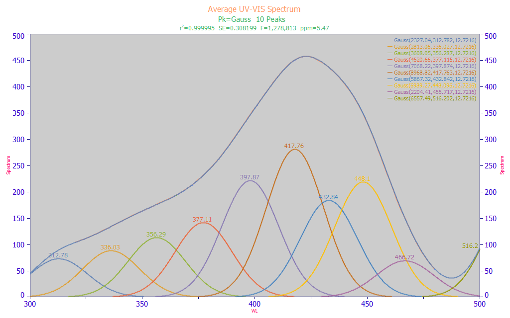
Click the Numeric button.
Fitted�Parameters
r2�Coef�Det DF�Adj�r2 Fit�Std�Err F-value ppm�uVar
0.99999453 0.99999370 0.30819875 1,278,813 5.47379293
Peak Type a0 a1 a2
1 Gauss 2327.04317 312.781753 12.7216043
2 Gauss 2813.06354 336.027026 12.7216043
3 Gauss 3608.05433 356.287029 12.7216043
4 Gauss 4520.65944 377.114717 12.7216043
5 Gauss 7068.21501 397.873914 12.7216043
6 Gauss 8968.81560 417.763054 12.7216043
7 Gauss 5867.31659 432.841836 12.7216043
8 Gauss 6989.27350 448.096465 12.7216043
9 Gauss 2204.41071 466.717086 12.7216043
10 Gauss 6557.48869 516.201847 12.7216043
The last of the peaks fails significance in its a0 area parameter (grayed), typical of partial peaks. The fitted Gaussian a2 width (SD) is 12.7 nm.
In this type of estimate, we performed a simple multiple Gaussian peak fit where we fit wavelength (nm) instead of frequency (cm-1) and where, by necessity, a single fitted width is shared across all peaks.
We perform this type of preliminary fitting to ascertain two important pieces of information. First, the width of the Gaussian peaks helps us to understand the spacing for the predictors used in the full permutation predictive modeling. In this case, a spacing of 5 nm is realistic, given this estimated peak width. If desired, the linear modeling algorithm can readily generate parameters further refined to the smallest wavelength spacing to see if a higher resolution in the final wavelengths offers any significant benefit. An x-spacing that is approximately half the Gaussian SD of the spectral peaks would be approximately 6 nm. Although the retained full permutation direct spectral fits rarely consist of fitting noise when the sample size is sufficient, such can still occur if the x-spacing is too narrow. Further, a high count of closely spaced predictors will produce seriously lengthy full permutation modeling times for no useful purpose.
Second, the center values of the fitted Gaussians represent wavelengths we might reasonably expect to see in the modeling. The peaks shown in this fit are only approximations, apply only to this averaged spectrum of all of the samples, and may not correspond exactly with the pure component absorbances which produce the overall spectra. This does, however, approximate what the linear modeling algorithms will be able to see and process. In this instance, we have three main UV wavelengths 336, 356, and 377 nm. There is one transition wavelength at 398 nm. There are four blue wavelengths at 418, 433, 448, and 467 nm. We will ignore the smallest and largest peaks in the fit above since they are outside the 320-480 nm modeling band.
The fit is a strong one, 5.47 ppm statistical (normalized least squares) error with an F-statistic of 1.28 million. We follow longstanding statistical modeling methodology where the highest value of the F-statistic is assumed to correspond with the maximum likelihood of the correct count of component peaks. From this fit, we would expect an effective predictive model to incorporate WLs close to these fitted a1 center values.
Please note that this type of peak fitting is not used in the predictive modeling. This type of preliminary analysis merely gives us a sense for the wavelengths we might expect to see in linear predictive models, as well as a reasonable wavelength spacing for fast full-permutation fitting.
Click OK to close the Peak Fit Review and return to the main window.
S/N of Spectra
To estimate the S/N of the UV-VIS spectra, we cannot use the average spectrum from the 156 samples. We must import individual spectra. We will import these directly from the spectral data matrix file that we will use for the modeling.
From the File menu's, Import Data Set(s), select the Import Data Sets from Model Data Matrix... item. Select the ModelingUVVIS_SpectralData.csv file from the program's installed default data directory (\PeakLab\Data).
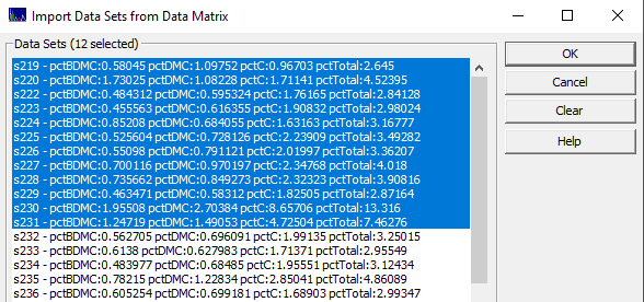
From the list, select the first twelve samples in the file, as above, and click OK.
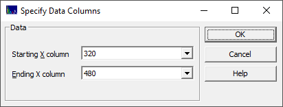
We will only import the data in the modeling band. Select 320 for the starting X-column, and 480 for the ending X-column. Click OK. Enter any name you wish, such as First12Spectra, for the file which will contain these twelve spectra. Click OK at the write notification. You will now see the first 12 spectra in the data matrix.
From the DSP menu, select the Fourier S/N Estimation... option.
If necessary, set the data taper window to None and be sure the Best Exact N Fourier algorithm is selected.
You will see the Fourier spectra for the 12 data sets. Click the Numeric Button.
S/N can be expressed as a ppm noise in the overall data, as decibel (dB) values, or by significant digits. We also measure the S/N in both the time and Fourier domains.
Signal Noise Analysis
Algorithm: Best Exact N
Window: None
Size Size Time Time Time Fourier Fourier Data
Data FFT SNRdb Digits ppm SNRdb Digits ID
161 161 41.3216935 2.06608467 8588.46056 58.5532309 2.92766154 s219
161 161 51.6809324 2.58404662 2605.87379 61.3382564 3.06691282 s220
161 161 41.9321351 2.09660675 8005.58819 65.2179760 3.26089880 s222
161 161 43.7644836 2.18822418 6482.99698 62.7763699 3.13881849 s223
161 161 45.0613650 2.25306825 5583.82435 63.0190151 3.15095076 s224
161 161 45.4617571 2.27308786 5332.27015 64.6110313 3.23055156 s225
161 161 45.5542386 2.27771193 5275.79691 65.2302258 3.26151129 s226
161 161 47.2975383 2.36487691 4316.41394 63.2402817 3.16201409 s227
161 161 47.4876148 2.37438074 4222.98228 61.9017618 3.09508809 s228
161 161 41.6075109 2.08037555 8310.44834 63.7479261 3.18739630 s229
161 161 55.0072352 2.75036176 1776.79875 65.4612237 3.27306119 s230
161 161 52.1091906 2.60545953 2480.50707 64.0886330 3.20443165 s231
Avg 46.5238079 2.32619040 5248.49678 63.2654943 3.16327472 All Data
For this data the time domain estimate of S/N is 2.33 significant digits. This is the point where half the precision is lost. The Fourier domain contributes the noise floor, the significant digits where all precision is lost, and this is 3.16 digits. Beyond 3.16 significant digits, this data is only noise. There is nothing exceptional about the S/N of the UV-VIS reconstructed spectra to justify a higher sampling density.
Close the Signal Noise Analysis numeric window and click OK to close the Fourier S/N procedure. From the File menu select Close to clear the current data.
Visualizing the Design Data Matrix
From the Model menu's Import Data Matrix item, select the Import Spectroscopic Data Matrix... option. We select the same data matrix file as above, s219-S372_UVVispt75-7m4(99)_Avg.csv in the PeakLab/Model folder. Answer No when asked if you wish to proceed to fit this data.
From the Model menu's Graph Data Matrix item, select the Graph All Data Sets in Spectroscopic Data Matrix... option. Again enter 320 for the starting X-column and 480 for the ending X-column and click OK.
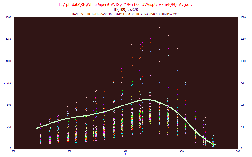
Check the Use Mouse button and highlight the individual data sets by passing the mouse over a given spectrum. In the above plot, a sample with a high UV signal and proportionately lower visible signal is highlighted. Click the Unit Area Normalization and place the mouse on the spectra that is furthest removed from all of the others.
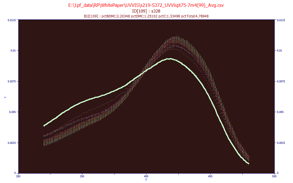
Here we see this same sample. The Unit Area format is useful for spotting significant differences in the spectral absorbances. Click OK to close the GLM matrix plot.
Direct Spectral Fit of Total Curcuminoids
Once the Import Data Matrix | Import Spectroscopic Data Matrix... item in the Model menu is used to load a spectroscopic modeling data matrix into the program, the Fit GLM Models option is available for fitting full-permutation GLM models, and for fitting smart stepwise forward models and sparse PLS models, both of which use the full permutation models as their starting point.
The PeakLab full permutation GLM models are an alternative to the PLS (partial least squares) and PCR (principal component regression) procedures.
From the Model menu, select the the Fit Full Permutation GLM Models... option. This is the entry point for all predictive modeling.
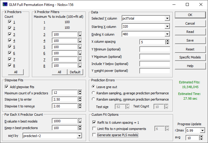
There are seven sections that govern the modeling.
X Predictors
We want to fit all of the X-predictors through the full eight allowed in the GLM full permutation algorithm. Click All in the X Predictors section to select all of the predictor counts if needed.
X Predictor Filters
We want to fit all of the WLs in the full permutation modeling, based on the X column spacing we will subsequently specify. Click All so that 100% (no filtering) is shown for all predictor counts.
Stepwise Fits
We will use the defaults. Be sure Add stepwise fits is checked, the Maximum count of x predictors is set to 12, the Stepwise t to enter is 2.50, and the Stepwise t to remove is 2.00.
For Each X Predictor Count
We will also use the defaults. Be sure Evaluate n best models is set to 1000, Keep n best predictions is 100, and the sort by is set to predicted r2. These numbers specify retaining the best 1000 models (by least squares error in the model fits) at each predictor count, evaluating them for the best r2 of prediction, and keeping 100 models for the GLM Review.
Data
Select the pctTotal column in the data file for the Selected Y column, 320 as the Starting X column, and 480 as the Ending X column. First, let's enter 1 for the X column spacing. You should see, in red, an estimate of 9.9 trillion fits. On a basic four core machine, this will require about 67 days. Change the X column spacing to 2, reducing the total WLs in the full permutation modeling from 161 to 81, The estimate should now be shown in magenta, and there are 36 billion fits. Again, on a basic machine, this will require about 5.8 hours. We know, from the peak fitting that the Gaussian width of the spectral absorbances is approximately 12 nm, and that a spacing much below 6 nm will not contribute to the prediction efficacy of the direct spectral models. Change the X column spacing to 5. This will use 33 total wavelengths in the full permutation modeling, and fit 19.5 million fits. For this basic four core machine, about 28 seconds will be required. We will use this 5 nm spacing.
Prediction Errors
Be sure the Leave One Out is selected.
Custom Fit Options
Check the Refit to X column spacing = 1. This will perform an additional fitting step to resolve the predictors to a 1 nm resolution.
Click OK to start the fitting.
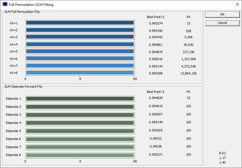
Because this is a rather basic modeling problem, even the 1-predictor fits have a very high predicted r2. Click OK when the fitting is done and choose a name for the saving the full fit information to disk. Using this file you can recall this fit in a single import step at any point further along. You will now see the GLM Review.
Reviewing the Direct Spectral Fits
The GLM Review assembles the full-permutation GLM models, the smart stepwise forward models, and the sparse PLS models for an intelligent selection of a final predictive model.
The two most important windows will be the Model List window and the main GLM Review window containing the model plot and significance map. The Model List window will initially look similar to the following. The models may be in a different order if you have changed the defaults.
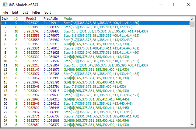
The default Model List settings will consist of displaying only the predicted r2 and predicted average error. In the List menu of the Model List window, select Median Error of Prediction. In the Filter menu, select Single Predictor Count and then select Include 8 Predictor Models. You see only the 8-predictor retained models. From this Filter menu, select Include 7 Predictor Models. You now see only the 7-predictor retained models. In the Sort menu, choose By X Predictor Compliance. This sorts the retained 7-predictor fits currently shown in the list by compliance with the weighted significance map of the all of the retained 7-predictor fits.
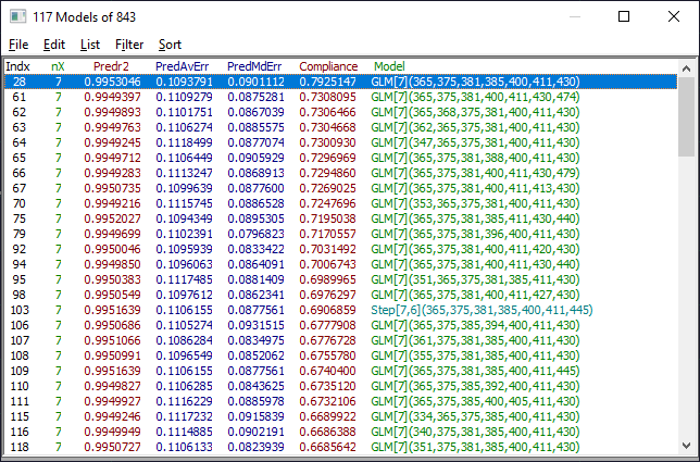
The list is now ordered by the models that best match the 7-predictor wavelength significances, weighted by prediction error, across all retained 7-predictor models. You can think of this as a kind of maximum likelihood of wavelengths across the most effective models.

The model plot shows this first selection in the Model List, the model containing the wavelengths most compliant in a prediction performance weighted average of significance for all 7-parameter models retained in the fitting procedure. The lower model plot has the reference Y values of the modeling on the X-axis, and the predicted values on the Y-axis. By default, the lower plot will also show a 95% prediction interval for a linear fit of that reference vs. predicted plot. The upper graph in the model plot is a residuals plot (difference between predicted and reference). The residuals are defined so that the directions match in the two plots. The background colors highlight the five quintiles in the Y-data of the modeling.
Note that the model with the best wavelength significance compliance is not normally the best performing model on any other prediction metric.
Predictor Count Optimization
Click the Fit Performance button in the main GLM Review window. Select Best Only.
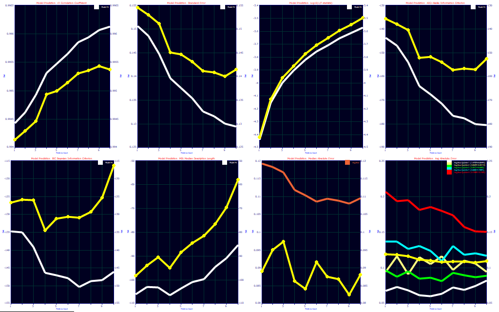
Multivariate parameter count optimization is an extensively studied science, and many different prediction metrics, or combination of metrics, are often used. The panels consist of r2 of prediction, standard error of prediction, base-10 log of F-statistic inverse, the corrected Akaike Information Criterion (AICc), the Bayesian Information Criterion (BIC), the Minimum Description Length (MDL), the median prediction error, and the average prediction error. The first six plots contain a reference (white curve) which contains the same metric for the model estimation or calibration. This metric from the design fit will almost universally be better than the prediction value. The median plot in the seventh panel has as its reference the average error (orange). The median error will almost always be lower than the average error. The average prediction error plot in the eighth panel has average prediction error references for the 5 quintiles of the Y-variable. In general, the average errors will tend to increase with the magnitude of the Y values.
![]() Click the Toggle Display of Reference Data button in the graph
toolbar of the Fit Performance graph.
Click the Toggle Display of Reference Data button in the graph
toolbar of the Fit Performance graph.
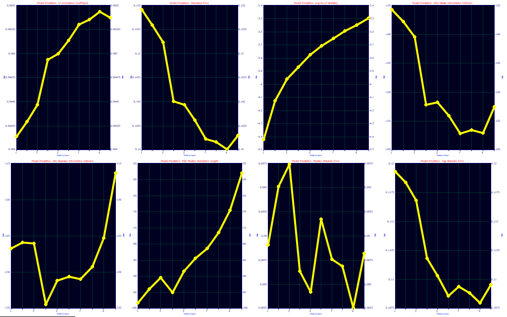
The choice of optimization is both art and science, and experience will often dictate your preference. We usually defer to an information criterion, but we like to see where the predictions level off for errors. In this fit, there are only small differences between a 1-predictor fit and higher predictors, and as such these optimization criteria are not consistent. The best prediction by r2, SE, median, and average error is with 9-predictor smart stepwise models. The F-statistic and MDL optimize to just 1 predictor, the AICC to 7, and the BIC to 4. In looking closely at the eight optimizations, we would tend to go with the 4 predictor, following the BIC. At 4 predictors, you have much of the r2, SE, median and average errors, the AICc flattens out at 4, and the MDL has a second minima at 4.
Click OK to close the Fit Performance Plot. In the Model List window's Filter menu, be sure the Single Predictor Count option is checked and select the Include 4 Predictor Models option. If the Sort is still set to By X Predictor Compliance, this is the model you should see:
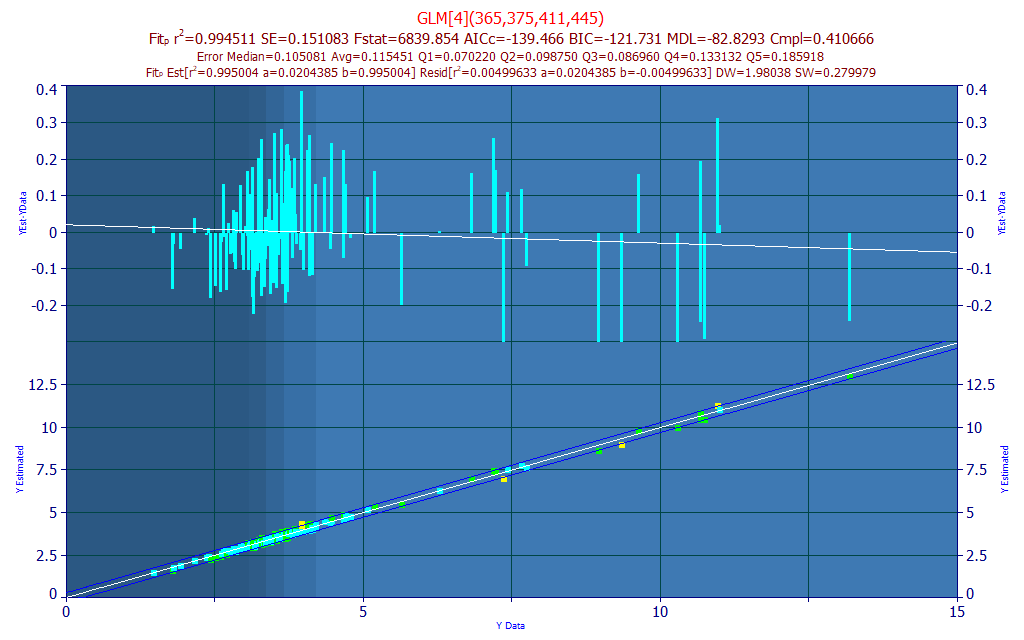
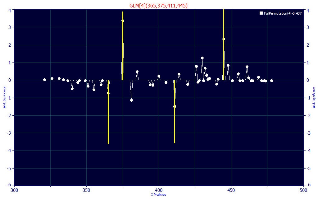
If we look at the first 4-predictor model, we see two UV and two VIS wavelengths. The 375 and 445 WLs generate the positive component of the prediction and the 365 and 411 WLs offset. We did see 377 nm and 448 nm in the peak fit we first made to identify target signal frequencies.
Experience and Judgment
In the initial visualization of the data matrix we saw one spectrum that was well removed from the others, nothing between. Is there another variant in nature not as yet included in our model data that would produce an equally strong deviation from the bulk of the spectra, but which would be as different or distinct? If so, there is a way to estimate that kind of error.
Click OK in the main GLM Review to exit the procedure and once again from the Model menu, select the the Fit GLM Models option. This time check the Random sampling, minimum prediction performance option for Prediction Errors. Leave the defaults in place (2/3 data to model, 1/3 data to blind prediction, 10 random sets). Click OK to refit the data, click OK when the fit has concluded, and enter a different file name for saving this fit to disk.
As a first step, click the Fit Performance button.
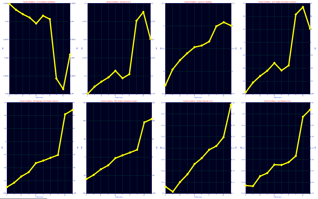
The Leave One Out prediction estimates allow for very little loss of bracketing in the modeling problem. Model bracketing issues are emphasized when using a worst-case error in a random sampling procedure. This assigns the highest error as opposed to an average when multiple blind predictions exist for a given sample. Note how different the optimizations look. The predicted r2 optimizes to 1 (9), the SE to 1 (9), the F-statistic to 1 (1), the AICc to 1 (7), the BIC to 1 (4), the MDL to 1 (1), the median error to 2 (9), and the average error to 2 (9). The Leave One Out predictor count optimizations are in parentheses. If you feel you are susceptible to an incomplete bracketing of the modeling problem in your design data, this kind of analysis may be helpful. Here it suggests that we may be better off with a single predictor model if we wish our prediction to defend against this kind of unknown.
Click OK in the Fit Performance window to close it. In the Filter menu of the Model List window, select Include 1 Predictor Models.
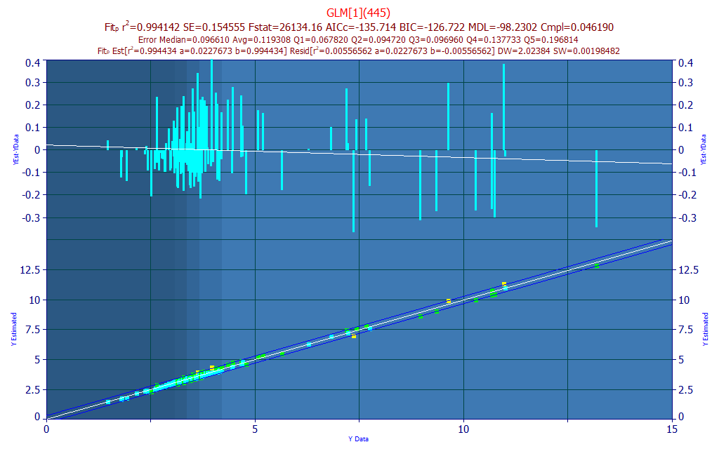
The best single predictor model, by r2 of prediction, is the one with the 445 nm wavelength, and the stats and errors are only slightly weaker (5858 ppm least-squares error vs 5489 for the 4-WL model).
Prediction
Click the Prediction button in the left panel of the GLM Review window. Select the file ModelingUVVIS_PredictionData.csv from the program's installed default data directory (\PeakLab\Data). . This file contains 602 spectra which were nowhere used in the modeling.
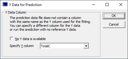
If the file containing the spectra for prediction doesn't have a matching Y-value name, you must select it if these spectra have known reference values. Select TotalC for the Y-column and click OK. A full Prediction procedure window opens and the model graph's upper plot is modified to show this prediction instead of the residuals from the leave one out prediction from the fitting.
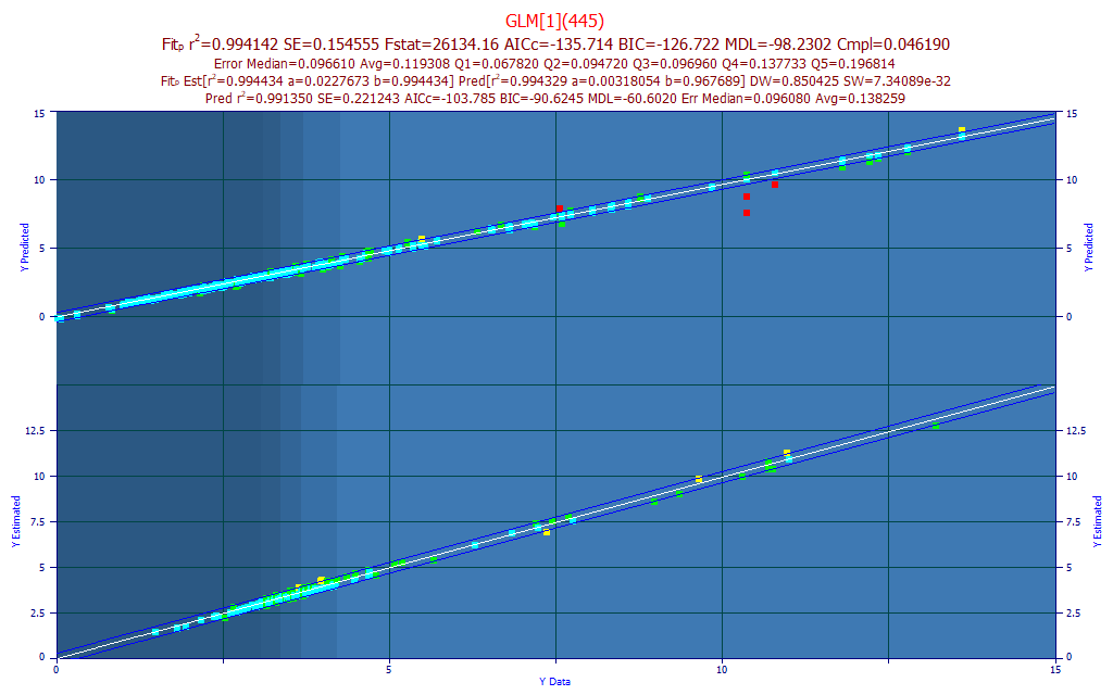
In this case, we see only a few outliers in the upper plot's prediction. The r2 of this different prediction is weaker, 0.9914 vs. 0.9941 for the leave one out prediction error estimated during the modeling.
Rank 733 GLM[1](445)
Prediction Statistics - from Original Fit - Leave One Out
Data: s219-S372_UVVispt75-7m4(99)_Avg.csv - 156 Observations
Fits: s219-s372_uvvispt75-7m4(99)_avg_nofilter_totalc_1nm.bin
Y Column in Data Matrix: 6 (pctTotal)
r2 SE F-stat AICc BIC MDL DOF
0.9941419 0.1545550 2.613e+04 -135.7143 -126.7226 -98.23023 154
Median Err Avg Err Avg Err Q1 Avg Err Q2 Avg Err Q3 Avg Err Q4 Avg Err Q5
0.0966062 0.1193078 0.0678179 0.0947165 0.0969568 0.1377332 0.1968144
Quintile Lower Upper
First 1.4797533 3.0649067
Second 3.0649067 3.3511367
Third 3.3511367 3.6682000
Fourth 3.6682000 4.1988067
Fifth 4.1988067 13.198050
Prediction Statistics - from Prediction Data
s001-218_SpectraWtAdj2_T123_m17(PI99).csv - 602 Observations
r2 SE F-stat AICc BIC MDL DOF
0.9913499 0.2212434 6.876e+04 -103.7852 -90.62456 -60.60203 600
Median Err Avg Err Avg Err Q1 Avg Err Q2 Avg Err Q3 Avg Err Q4 Avg Err Q5
0.0960807 0.1382589 0.0906968 0.1154860 0.1391623 0.1389409 0.2568171
Prediction Statistics - 10 Outliers Removed
s001-218_SpectraWtAdj2_T123_m17(PI99).csv - 592 Observations
r2 SE F-stat AICc BIC MDL DOF
0.9946643 0.1601656 1.1e+05 -484.4910 -471.3813 -439.9328 590
Median Err Avg Err Avg Err Q1 Avg Err Q2 Avg Err Q3 Avg Err Q4 Avg Err Q5
0.0935228 0.1235726 0.0906968 0.1154860 0.1391623 0.1389409 0.1952699
The prediction window will help you see if a prediction stands up to blind data. For this one-predictor model, we see an average leave one out prediction error of 0.1193. The predictions from the new data have an average error of 0.1382 with the red points included. By default, the prediction procedure trims out predictions outside of 3 SE of the reference fit. In this case, 10 possible outliers were removed and the average error dropped to 0.1235, respectably close to the leave one out error from the modeling. In general, you should expect some measure of incomplete bracketing in the model data relative to fully blind prediction data. We see that here, although this is small - what prediction scientists want to see.
In the Prediction window's Outliers menu, choose Outside of 2 SE in the Multiples of SE.
Prediction Statistics - 36 Outliers Removed
s001-218_SpectraWtAdj2_T123_m17(PI99).csv - 566 Observations
r2 SE F-stat AICc BIC MDL DOF
0.9952925 0.1376405 1.192e+05 -634.6026 -621.6296 -589.8934 564
Median Err Avg Err Avg Err Q1 Avg Err Q2 Avg Err Q3 Avg Err Q4 Avg Err Q5
0.0885558 0.1103185 0.0869513 0.1154860 0.1285117 0.1248069 0.1582827
With this stricter removal of potential outliers, the count of predictions has dropped by another 26 spectra and the average prediction error from these 566 remaining spectra is now .1103.
Scroll through the Model List while looking at the Prediction window and in particular, note the median error with no outliers removed.
Click OK to close the GLM Review.
Comparison with PLS and PCR
Partial Least Squares (PLS) and Principal Component Regression (PCR) are often used in chemometric modeling. How did our full permutation direct spectral modeling in this example compare?
The Unscrambler software application automatically selects the 1-factor PLS when fitting 320-480 at a 1 nm spacing. This 1-factor PLS model, has a 0.992103 r2 prediction (7893 ppm error), an average absolute prediction error of 0.135, and a median absolute prediction error of .115. The optimum PLS by best Leave One Out r2 of prediction is a four factor model:
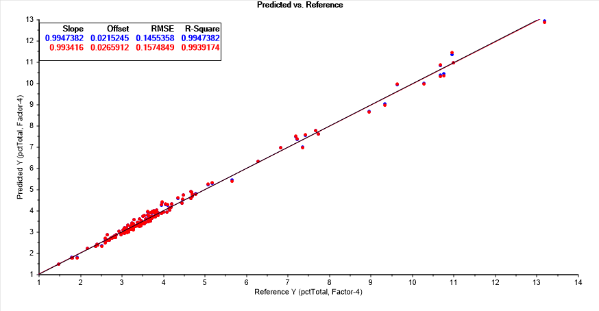
This PLS model, 4-factor, 161 wavelengths, 162 coefficients, has an r2 prediction of 0.993917 (6083 ppm error), an average absolute prediction error of 0.115, and a median absolute prediction error of .929.
The optimum PCR by a Leave One Out r2 of prediction is a five principal component model. This PCR model, 5-principal components, 161 wavelengths, 162 coefficients, has an r2 prediction of 0.993896 (6104 ppm error), almost identical to the best performing PLS model by the Leave One Out prediction method, an average absolute prediction error of 0.117 and a median absolute prediction error of .934.
In this specific modeling problem, the direct spectral fits, even the simple 1-predictor model, outperformed the best PLS and PCR models.
A More Challenging Modeling Problem
In the Modeling Spectra - Part I - UV-VIS Data white paper, we discuss the challenges associated with fitting the bis-demthoxycurcumin (BDMC) in the UV-VIS.
Click OK in the main GLM Review to exit the procedure and once again from the Model menu, select the the Fit GLM Models option. Once again check the Leave One Out Prediction Errors and change the Selected Y Column to pctBDMC. Click OK to refit the data.
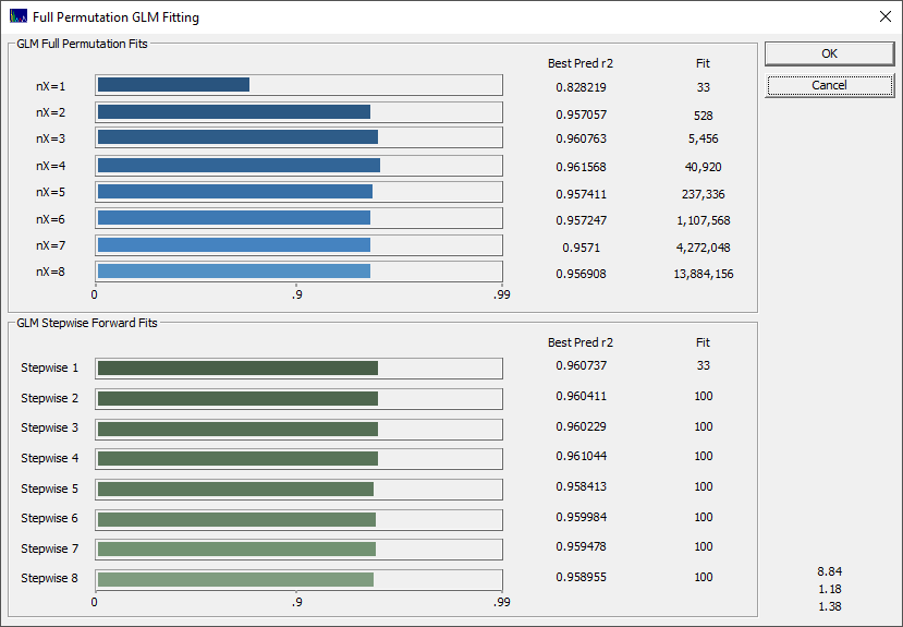
You will note a very different look to the progress bar, and there is an indication the average of the best 10 r2 of prediction models occurs with 4 predictors.
Click OK when the fit has concluded, and enter a different file name for saving this fit to disk.
As a first step, click the Fit Performance button.
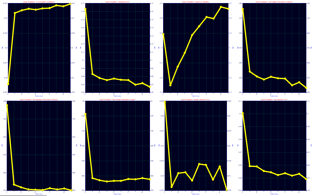
If you look closely at the BIC in the fifth panel and the MDL in the sixth you will see that both show an optimum at 4 predictors.
Click OK to close the Fit Performance Plot, In the Model List window's Filter menu, be sure the Single Predictor Count option is checked and select the Include 4 Predictor Models option. In the Sort menu, select By X Predictor Compliance.
![]() Click the Select Color
Scheme and Customize
Colors button in the graph's
toolbar. Select the Cyan color scheme and click OK. This is the model you should
see:
Click the Select Color
Scheme and Customize
Colors button in the graph's
toolbar. Select the Cyan color scheme and click OK. This is the model you should
see:
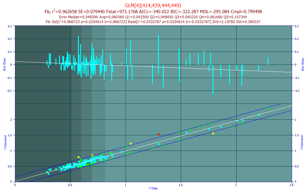
The errors are much smaller in magnitude only because there is far less BDMC in most turmeric samples. The r2 of prediction is much weaker. The red points in the model plot are those where the absolute residual is greater than 3 standard errors of this linear fit between the measured and predicted. There is one spectrum amongst the 156 that is outside 3 SE. The yellow points in the model plot are those outside 2 SE. There are four such spectra.
We will first get a sense for what a fit might look like if these red and yellow spectra points in the lower model plot were treated as outliers, where the measurements are treated as suspect, and these were removed from the data and a refit was made.
Click Prediction in the left panel of the GLM Review window and select the same s219-S372_UVVispt75-7m4(99)_Avg.csv file we used for the modeling. In doing this, we have only used the Prediction feature to replicate the model plot. Right click the model plot and select the Mark Inactive Outside Prediction Interval option.
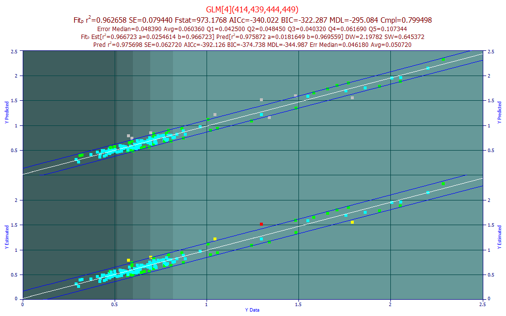
The last line in the titles and the upper plot reflect an improvement in the linear fit from 0.9667 to 0.9757 by the removal of points outside the default 95% prediction interval (this interval can be changed in the graph toolbar). Note that eight spectra were removed by this prediction interval criterion. If we felt that these truly were outliers in the data, we could use the Data option to flag outliers using any number of statistical criteria, and we could then utilize its File menu Save Data w/Flagged Outliers Removed option to save a revised data matrix without these spectra present. The revised data matrix would then be fitted. In this instance, we believe the wider error band is more likely due to the difficulty in modeling this component. Even if certain BDMC estimates are outliers from a measurement error, their exclusion will not get us anywhere near the accuracy seen in the total curcuminoids model.
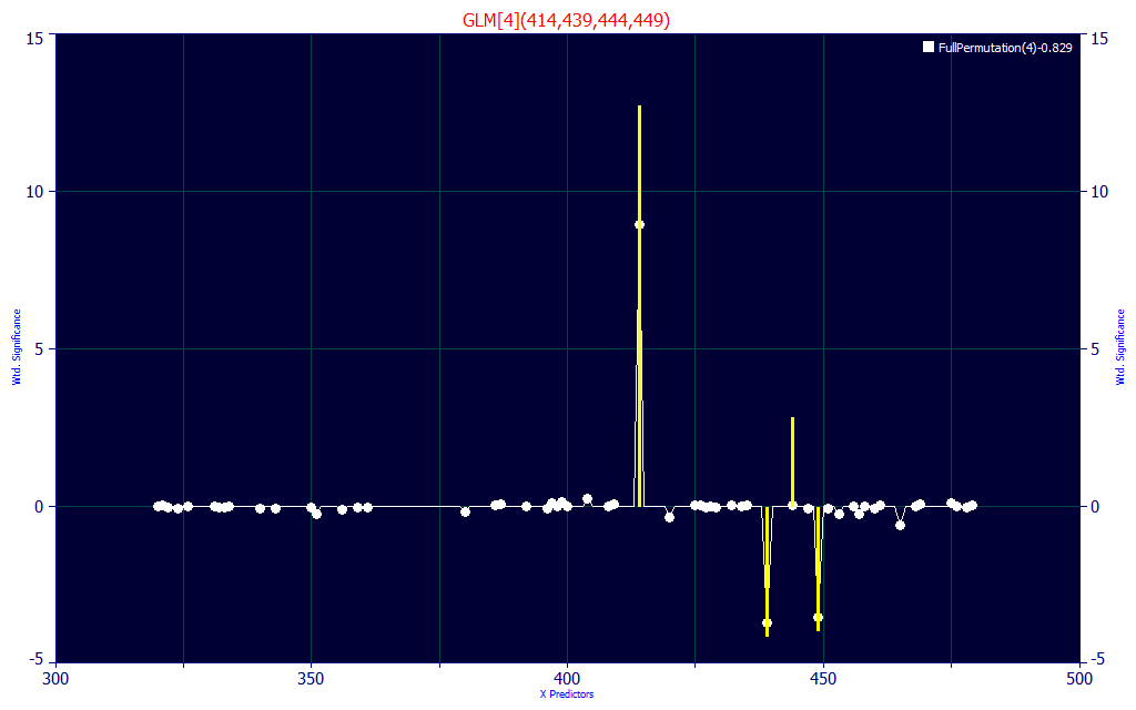
The model we are looking at has its principal positive contribution at 414 nm. In the Modeling Spectra - Part I - UV-VIS Data white paper Fig. 5, we demonstrate that the BDMC central peak is at a 417 nm blue absorbance and its chromatographic coeluting companion is at about 412 nm. The 414 central WL makes sense, as do the offsets between 435-450 nm that address the zone where the three components are most strongly separated.
In this model, no UV WLs at all were used.
Click the Significance button in the left panel of the main GLM Review window, and select Contour if it is not already selected. Zoom the contour plot to show only the 3-8 predictor models.
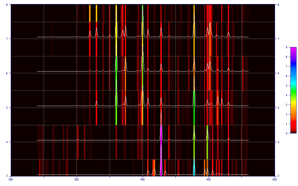
In the contour map, the UV wavelengths do not have a strong presence until 5 predictors are used in the models. Note that the five and higher predictor models have a very different significance map with respect to the four predictor models.
Click OK in the Significance window to close it. In the Model List window's Filter menu, be sure the Single Predictor Count option is checked and select the Include 5 Predictor Models option. In the Sort menu, select By X Predictor Compliance.

The compliance brought 5-predictor models with one or more UV wavelengths to the top of the list. This first model in the list has an r2 of prediction that is weaker, even though the median and average errors are less. If you look closely at the quintile 5 (Q5) average prediction error, you will see that it is appreciably higher in this model. This fifth quintile has the lightest color background in the plot and consists of the samples with the highest BDMC content.
We will filter the list so that only models with 400-450 nm visible wavelengths are shown. In the Model List Filter menu, select No Filter to clear all filtering. In the Sort menu, choose By Predicted r�. From this same Filter menu, select Custom X Band Filtering.
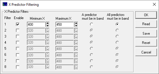
Enter the filter as above and click OK. Select the 2nd model in the list, the Rank 2 Step[5,4](414,420,444,447,449) model. This is a stepwise model that incorporates a great deal of tail information for the visible spectral feature.
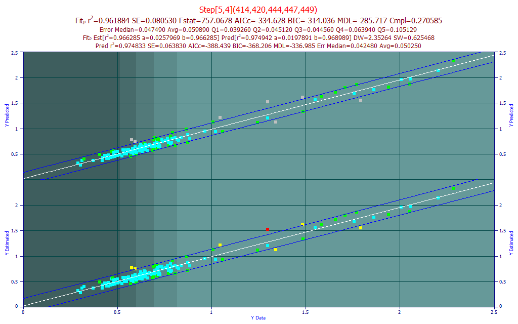
Did we benefit from this additional predictor versus the 4-predictor model? The r2 of prediction is weaker, the F-stat is appreciably less, and there was no significant improvement in any of the errors.
In the Model List Filter menu, select No Filter to clear the custom filtering and then select the Include 4-predictor Models. Our four-predictor model is again shown.
Exporting the Model
It is a simple matter to export the selected model.
C++
Click Numeric, and in the Numeric Summary window's Options menu, select the C++ Code - Input Specific X-Predictors. You will see the following at the bottom of the Numeric Summary:
C++ Language Code - argument is specific spectra
double glm01(double *spec)
{
// spec[0] X Predictor 1 (414, index=94)
// spec[1] X Predictor 2 (439, index=119)
// spec[2] X Predictor 3 (444, index=124)
// spec[3] X Predictor 4 (449, index=129)
double p[5]= {
0.0221445801426611, 0.0202444570210056, -0.01915233028586, 0.0189152012010083, -0.021939480431503,
};
int nx = 4;
double estimate = p[0];
for(int i=1; i<=nx; i++)
estimate += p[i]*spec[i-1];
return estimate;
}
The model is as simple as storing the constant and performing a dot product with four coefficients and four spectral values.
Visual BASIC
In the Numeric Summary window's Options menu, select the VB Code - Input Specific X-Predictors. You will now see the following at the bottom of the Numeric Summary:
VBA - Excel - specific spectra across columns in a single row
Function GLMEval(Spectra As Range) As Double
' Spectra in Spectra.Cells(1,1) X Predictor 1 (414, index=95)
' Spectra in Spectra.Cells(1,2) X Predictor 2 (439, index=120)
' Spectra in Spectra.Cells(1,3) X Predictor 3 (444, index=125)
' Spectra in Spectra.Cells(1,4) X Predictor 4 (449, index=130)
Dim N As Integer
Dim i As Integer
Dim eval As Double
Dim parms(21) As Double
parms(1) = 0.0221445801426611
parms(2) = 0.0202444570210056
parms(3) = -0.01915233028586
parms(4) = 0.0189152012010083
parms(5) = -0.021939480431503
eval = parms(1)
N = 4
For i = 1 To N
eval = eval + Spectra.Cells(1, i) * parms(i + 1)
Next i
GLMEval = eval
End Function
This code is structured to work within the VBA Excel development environment.
Excel In-Cell Formulas
Click the Data button in the left panel of the main GLM Review window and from the Data window's File menu, select Save Summary And X Data As... option. Save the CSV file, and if you wish, open this CSV file in Excel.

In this export, the formula in cell L2 is a string. Convert it to a formula with a leading = symbol and copy it to the additional rows in the L column where there is spectral data in the G-J columns

Column L now contains the model evaluations matching the results you see in the Data summary.
Evaluating the Prediction in Various Applications
The Prediction should still be shown in the upper plot in the GLM Review graph. Right click the graph and choose Refresh - Clear Inactive. The upper Prediction plot and the lower Model plot should now match. All of the following options will allow you to validate the models in other application software.
Maple
In the Prediction window's Edit menu select Copy Prediction Evaluations for Maple.
Parms:=[-0.049541042518362,0.011068653042172]:
WL:=[445]:
mSpec:=[[1,382.708145121588],
[1,398.806969759026],
[1,370.069754244102],
...
[1,275.992993955259],
[1,240.21593729655]]:
pred :=array(1..602):
for i from 1 to 602 do
p := 0: for j from 1 to 2 do p := p + mSpec[i,j]*Parms[j]: od:
pred[i] := p:
od:
print(pred);
Paste this code into Maple to evaluate all of the spectra imported in the prediction.
Mathematica
In the Prediction window's Edit menu select Copy Prediction Evaluations for Mathematica.
Parms:={-0.049541042518362,0.011068653042172}
WL:={445}
mSpec:={{1,382.708145121588},
{1,398.806969759026},
{1,370.069754244102},
..
{1,275.992993955259},
{1,240.21593729655}}
Table[mSpec[[i ;; i, 1 ;; 2]].Parms, {i, 1, 602}]
Paste this code into Mathematica to evaluate all of the spectra imported in the prediction.
Excel
In the Prediction window's Edit menu select Copy Prediction Evaluations for Excel. You can also use the Prediction window's File menu option Save Summary and X-Predictor Data As... to write this information to a CSV file. It is similar to the the Data window's File menu Save Summary And X Data As... option except that the imported prediction data is written to the file.
C++
#include "stdafx.h"
double Parms[2]={-0.049541042518362,0.011068653042172};
double WL[1]={445};
double mSpec[602][1]={
{382.708145121588},
{398.806969759026},
...
{275.992993955259},
{240.21593729655}};
double glmEval(int nx, double *parms, double *spec)
{
double estimate = parms[0];
for(int i=1; i<=nx; i++)
estimate += parms[i]*spec[i-1];
return estimate;
}
double *glmEvalAll()
{
int nobs = 602;
int nx = 1;
double *estimate = (double *)calloc(nobs, sizeof(double));
for(int i=0; i<nobs; i++)
estimate[i] = glmEval(nx, Parms, mSpec[i]);
return estimate;
}
The glmEvalAll() function will evaluate all of the predicted data, glmEval(_) evaluates a single prediction.
Click OK to close the GLM Review.
Modeling Spectra Tutorial II - Powder FTNIR
In the second modeling tutorial, we will address spectral data that is far harder to model. We address both obfuscating absorbances, as well as latent variables of powder particle size (distribution density) and powder moisture content.